is the kth sequence. If each sequence is independent of all others, then we should have: ¯aij = âK k=1 .... John. Wiley & Sons, New York, 1989. [5] H. von Helmholtz. Popular Scientific Lectures, chapter The ... [10] J.K. Tsotsos. On the Relative ...
On the Visual Expectations of Moving Objects Shaogang Gong∗
Hilary Buxton?
Computer Science Department, Queen Mary and Westfield College, Mile End Road, London E1 4NS, England Abstract. Meaningful objects in a scene move with purpose. In this work, a Hidden Markov Model is used to represent the “hidden” regularities behind the apparent object movement in a scene and reproduce such regularities as “blind” expectations. By adapting the weights on beliefs with new visual evidence, an Augmented Hidden Markov Model is used to produce dynamic expectations of moving objects in the scene. Keywords: Visual observation, tracking, visual expectation and visual attention, learning, probabilistic belief network, augmented Hidden Markov Model.
1
Introduction
Vision is highly selective [4, 1], purposive [5] and active [3]. Task knowledge and the nature of the scene often define the visual attention and allow us to ignore the irrelevant [4]. In visual observation, understanding and interpreting moving objects in the scene is a conscious behaviour such that hypotheses and expectations of the moving patterns of objects being observed are made constantly [5]. It is for such reasons that we address in this work the problem of how moving objects in a scene can be observed with expectations in order to provide cues for selective visual attention. Similar work has been addressed by [2, 9, 10]. Meaningful objects always move with purposes. In a known environment, such inherent purposes are associated with patterns of moving sequences which are constrained by the spatio-temporal characteristics of the environment. Moving purposes of an object is often distinctively captured by the spatio-temporal regularities in its movement patterns. A common phenomena would be the observation of service vehicles entering an airport docking stand (figure 1). The hidden regularities can be regarded as a set of conditional dependencies in space and time and such spatio-temporal dependencies are mostly qualitative and probabilistic. Inspired by Rimey and Brown’s recent study in active vision [8], we extend the use of
? The work is funded by the ESPRIT EP2152 (VIEWS) project.
Augmented Hidden Markov Model to model the probabilistic spatio-temporal regularities in object’s movement for providing visual expectations and selective visual attention.
2
“Blind” Expectations
Hidden Markov Model (HMM) has been widely used in speech recognition for modelling and classifying sound patterns. A HMM is essentially defined by its initial state probability distribution π, the symbol probability distribution B and the state transition probability distribution A. A HMM represents the probabilistic characteristics of a sequential pattern in two levels: (1) a state sequence represents a sequential combination of “hidden” hypotheses; (2) an observation symbol sequence models the most likely combination of local evidence for the transitions between the states. A detailed overview of HMM can be found in [7]. In figure 1, when a vehicle enters the scene, the spatial locations at which significant changes in orientation of vehicle’s movement occur are the states. The visual evidence, orientation and displacement of the vehicle’s movement, are the symbols. Assuming that there is only a very weak correlation between the orientation and the displacement of vehicle’s movement, we can use a pair of independent HMMs to model the orientations and displacements simultaneously. In other words, a HMM can be applied to capture the probabilistic moving regularities of a type of vehicle. The probability distributions of a HMM are learned from examples. Provided with training sequences, multiple HMMs can be established for giving probabilistic spatio-temporal expectations of different vehicle appearances (see figure 2). The essence in HMM learning can be characterised as a process of establishing impacts of updated visual evidence from the training sequence on the model’s partial conditional beliefs 1 . More precisely, to compute: (1) the conditional probabilities of the partial observation sequence O1 , O2 , ..., Ot and state to be in 1 An excellent systematic analysis of graph-based belief networks can be found in [6].
Figure 1: Moving patterns of service vehicles at an airport docking stand. (1) a fuel tanker and a trailer in
service; (2) moving patterns of typical service vehicles in the ground plane; (3) 30 training sequences for the fuel tanker and (4) overlapped discrete orientations and the associated frame-wise displacements of the tanker. qi at time t, given the model, αt (i) = [
N X
αt−1 (j)aji ]bi (Ot )
(1)
j=1
where α1 (i) = πi bi (O1 ), 1 ≤ i ≤ N , 2 ≤ t ≤ T − 1; (2) the conditional probabilities of the partial observation sequence Ot+1 , Ot+2 , ..., OT , given the state had been in qi at t and the model, βt (i) =
N X
aij bj (Ot+1 )βt+1 (j)
mate of HMM λ can only be obtained through multiple learning sequences. Let us denote a set of K learning examples as O = [O(1) , O(2) , ..., O(K) ], where (k) (k) (k) O(k) = [O1 , O2 , ..., OTk ] is the kth sequence. If each sequence is independent of all others, then we should have:
PK a ¯ij =
(2)
PTk −1
PK
t=1
1 k=1 Pk
PK
j=1
where T is the length of the sequence, βT (i) = 1 and 1 ≤ i ≤ N , t = T − 1, T − 2, ..., 1. Based on equations (1) and (2), Baum-Welch learning algorithm [7] adjusts the probability distributions for a single learning observation sequence. However, a reliable esti-
1 k=1 Pk
¯bj (l) = Pk=1 K
1 Pk
PTk −1 t=1
PTk −1
1 k=1 Pk
where
½ dt =
1 0
(k)
k αkt (i)aij bj (Ot+1 )βt+1 (j)
t=1
αtk (i)βtk (i) dt αkt (i)βtk (i)
PTk −1 t=1
αkt (i)βtk (i)
if Ot = Vk otherwise,
,
(3)
Figure 2: The appearance of a fuel tanker initialises a visual blind expectation of future movement of that
vehicle. After 9 frames, a similar blind expectation was caused by the appearance of a fuel trailer. The next 4 ground plane diagrams show the positions of the vehicles at every 20 frames interval overlapped on the initial expectations. Pk =
P [O(k) |λ] =
N X
αTk (i)
(4)
duce vk at time t+1, then a belief modification weight is [8]:
i=1
3
atij btj (k) , ωjt = PN at bt (k) l=1 il l
Visual Expectations
Visual observation can be regarded as an ongoing process of adjusting our underlying expectations of object behaviour with instantaneous updated visual evidence and simultaneously applying such modified expectations to guide the visual perception in order to guarantee the effectiveness and correctness of future visual evidence (see figure 3). Visual augmentation on HMM was introduced for foveation control in active visual sensing [8]. The concept extends naturally to visual observation. Now, consider that: (1) the partial conditional beliefs are functions of time, i.e. we have λ(t) with a particular value at time t denoted as λt ; and (2) the updated visual evidence of the moving object is regarded as the immediate prediction of the λ(t)’s symbol output. That is, if i is the index of the state qi determined by λt at current time t, k is the index of the observation symbol vk at time t, and assuming that λt+1 will pro-
1≤j≤N
(5)
ωjt represents a conditional belief that λ(t) will be in state qj at time t + 1, given λt is in state qi and has received visual evidence for output symbol vk at time t + 1. Assuming that symbol vk will be generated by λt+1 , this conditional belief weighting factor gives approximately the state transition probability a ˜t+1 at ij t+1 t 2 time t + 1, i.e. a ˜ij = ωj where 1 ≤ j ≤ N . Once again, applying the same assumption that current visual evidence vk will be the immediate future output symbol of λ(t), and considering that this conditional belief is also dependent on the probability of λ(t) being in a particular state, we have: wjt dtj (l) ˜bt+1 , (l) = PM j wt dt (m) m=1 j j 2A
1≤l≤M
detailed analysis can be found in [8].
(6)
INTERPRETATION Classification and Interpretation of Changes
Visual Input
Model Expectation
Visual Evidence PREDICTING Modelling Expectations of What and Where to See
SEEING Tracking Changes in the Scene from the Images
Camera
Visual Alert Visual Focus ATTENTION Provide Selective Attention for Seeing
Model Expectation
Figure 3: A “see-predict-see” feedback loop in visual
observation. where
½ dtj (l)
=
1 0
if l = k otherwise
Further, considering that changes to the atij and btj (l) should be taken gradually, therefore controlled by a modification gain, and such changes can only be maintained if the same visual evidence is maintained, i.e. controlled by a decay gain, then: at+1 = rdg [rmg ωjt + (1 − rmg )atij ] + (1 − rdg )atij (7) ij bt+1 (l) = j sdg { PM
smg wjt dtj (l) + (1 − smg )btj (l)
m=1
[smg wjt dtj (m) + (1 − smg )btj (m)]
}+
(1 − sdg )btj (l) (8) where rmg and smg (0 ≤ rmg , smg ≤ 1) are state and symbol modification gains, rdg and sdg (0 ≤ rdg , sdg ≤ 1) are state and symbol decay gains respectively. As there is no visual evidence for the initial time step, the initial state distribution π cannot be adjusted.
4
Experiments and Discussions
Figure 2 shows blind expectations after the appearances of a fuel tanker and a fuel trailer have been detected. The length of the expectation is determined by the probability P [O|λi ] given by equation (4). Figure 4 shows the visually augmented expectations. It is evident that the expectations for the immediate future 20 frames are more accurate than for the distant future as the instantaneous visual evidence only influences expectations locally in time. It is also evident that under the current circumstance, no direct effect
exists on the visual tracking from which visual evidence is provided. An assumption was made that visual evidence at each time frame was collected under the guidance of the expectation. Our immediate future work will be on establishing this visual feedback link illustrated in figure 3. We described the need to have visual expectations for selective attention in visual observation and, more importantly, that selective attention should be context dependent. We illustrated how Augmented Hidden Markov Models can be used to capture the intrinsic spatio-temporal regularities of moving vehicles in a known scene and consequently, to predict vehicle’s movement with instantaneous visual augmentation. In this airport scenario, scripts are used to describe the expected vehicle service steps in loading and delivering. By linking the discrete “hidden” states of AHMM to the steps in the scripts, we should be able to deliver meaningful conceptual descriptions of the vehicle behaviour.
References [1] D. Ballard. Reference Frames for Animate Vision. In IJCAI, Detroit, USA, Aug. 1989. [2] P.J. Burt. Smart Sensing in Machine Vision. In Machine Vision: Algorithms, Architectures and Systems. Academic Press, San Diego, Ca., 1988. [3] J.J. Gibson. The Perception of the Visual World. Greenwood Press, Westport, CT, USA, 1950. [4] I.E. Gordon. Theories of Visual Perception. John Wiley & Sons, New York, 1989. [5] H. von Helmholtz. Popular Scientific Lectures, chapter The Recent Progress of the Theory of Vision. Dover Publications, New York, USA, 1962. [6] J. Pearl. Probabilistic Reasoning in Intelligent Systems, Networks of Plausible Inference. Morgan Kaufman Publ. Inc., Los Altos/CA, 1988. [7] L.R. Rabiner. A Tutorial on Hidden Markov Models and Selected Applications in Speech Recognition. Proceedings of the IEEE, 77(2):257–286, 1989. [8] R.D. Rimey and C.M. Brown. Selective Attention as Sequential Behavior: Modeling Eye Movements with an Augmented Hidden Markov Model. In DARPA Image Understanding Workshop, pages 840–850, Pittsburgh, USA, Sept. 1990. [9] T.M. Sobh and R. Bajcsy. Visual Observation as a Discrete Event Dynamic System. In IJCAI Workshop on Dynamic Scene Understanding, Sydney, Australia, Aug. 1991. [10] J.K. Tsotsos. On the Relative Complexity of Active vs. Passive Visual Search. International Journal of Computer Vision, 7(2):127–141, 1992.
Figure 4: The same scenario as in figure 2 but with visual augmentation at each frame. The gains from the
visual augmentation are smg = 0.1, sdg = 0.1, rmg = 0.4 and rdg = 0.4. The state transition gains should always be much smaller compared with the observation symbol gains because the instantaneous visual evidence at each frame should not have strong influence on the changes in its movement pattern. Also, because the current see-predict-see loop still lacks the “Visual Focus” and “Model Expectation” links shown in figure 3. Therefore, the confidence in the visual evidence under the current circumstance is low and all the gains for the augmentation have been set low.