ON TOLERATING FAULTS IN NATURALLY REDUNDANT ALGORITHMS* Luiz A. Laranjeirat Miroslaw Malekl Roy Jeneveins
Department of Electrical and Computer Engineering The University of Texas at Austin Austin, Texas 78712, USA Abstract A class of algorithms suitable f o r fault-tolerant execution in multiprocessor s y s t e m s by exploiting the existing embedded redundancy in the problem variables is characterized in this paper. Because of this unique
In this paper we characterize a class of algorithms, that need no hardware replication and require very small execution time overhead in order to provide redundancy for fault recovery, and sometimes for fault detection, too. This is possible due to a unique property these algorithms present, natural redundancy in the problem variables. Furthermore, the type of recovery this natural redundancy enables, forward recovery [l],can cause lower performance degradation than other recovery techniques such as checkpointing and rollback [2], besides not requiring massive hardware replication as fault masking techniques such as NMR (N-Modular Redundancy) [3]. In order to achieve fault tolerance with this class of algorithms it is still necessary to add explicit procedures to use the available redundancy for fault recovery and detection, and to implement schemes for fault location. Redundancy for fault recovery (and sometimes for fault detection), however, comes for free, and this is the most salient feature of the method we are proposing. Other advantages of our approach include the simplicity of the software-implemented schemes necessary for detecting faults and recovering the missing correct computational values. Other methods that can tolerate hardware faults through software-based schemes include selfstabilizing algorithms [4], inherently fault-tolerant algorithms [5] and algorithm-based fault tolerance [6]. The approach exploited in this research can tolerate a broader range of sin le processor faults (both permanent and temporary? with less performance degradation than self-stabilizing and inherent fault-tolerant algorithms, and with no need of algorithm redesign for providing redundancy for fault recovery as in algorithm-based fault tolerance. Although the proposed technique could be applied to both single and multiple processor architectures, we focus on multiprocessors where fault-tolerant algrithms are very necessary due to the increased probability of faults. The extra hardware existing in a multiprocessor system increases the probability of oc-
property, n o extra computations need be superimposed t o t h e algorithm in order t o provide redundancy f o r fault recovery, as well a s fault detection in s o m e cases. A forward recovery s c h e m e is thus employed with very low t i m e overhead. T h e method is applied t o t h e implementation of t w o iterative algorithms: solution of Laplace equations by Jacobi's method and the calculat i o n of the invariant distribution of a Markov chain. Experiments show less t h a n 15% performance degradation f o r significant problem instances in fault-free situations, and as low as 2.43% in s o m e cases. T h e extra computation tame needed f o r locating and recovering f r o m a detected fault, does not exceed the t i m e necessary t o execute a single iteration. T h e fault detection procedures provide fault coverage close t o 100% f o r faults causing errors that affect the correctness of the computations.
1
Introduction
It is a well known fact that redundancy is a necessity in the design of fault-tolerant systems. Therefore, a greatly important goal in this research area is how to provide the necessary redundancy for a system to be able to execute reliably with minimum overhead in terms of space (including hardware and software) and execution time. 'This research was supported in part by ONR under Grant N00014-88-K-0543 and NASA under Grant NAG9-426. 1Phone: (512) 471-1658, Email:
[email protected] f On leave at the Office of Naval Research in London. Phone: (44)(71)4044478, E m a i l :
[email protected] §Phone: (512) 471-9722, Email:
[email protected]
CH3021-3/91/~/0118/$01.000 1991 JEEE
I18
algorithm would potentially be able to recover more than one erroneous y i .
currences of failures, and consequently of faults, as well as provides the potential for tolerating them. In the body of this paper we will define Naturally Redundant Algorithms and show that they are well suited t o exploit this potential. We illustrate the application of our method with two iterative synchronous algorithms: solution of Laplace equations by Jacobi’s method and the computation of the the invariant distribution of a Markov chain. The experimental results show a performance degradation of less than 15%, and as low as 2,43% in some cases, in the fault-free execution of the algorithms for significant problem sizes. When a fault occurs it is located and recovered from with a performance penalty no larger than the execution time of a single iteration. The target architecture for our experiments was a Sequent Symmetry multiprocessor (see Section 3) in which we considered that the bus is fault-free and that memory faults are taken care of by error detecting/correcting codes. Our method would also be amenable for implementation in a distributed environment with some inexpensive modifications. In such case the fault coverage would be larger and the performance degradation higher when recovering from faults see Section 3). A c e a r disadvantage of our method is that it is application-dependent rather than general. We also assume that the sofwtare is correct, that is, the proposed technique aims t o tolerate processor faults. Even though single faults are the ones that can always be tolerated with our method, in some cases multiple faults could also be covered (see Section 4.3). In the next section we state some definitions and Section 3 describes the target architecture and the utilized fault model. Sections 4 and 5 detail how natural redundancy was exploited to provide fault tolerance in our examples. Section 6 presents the results of our experiments and Section 7 states our conclusions.
In the parallel execution of many applications processors communicate their intermediate calculation values to other processors as the computation proceeds. In such cases, the erroneous intermediate calculations of a faulty processor can corrupt subsequent computations of other processors. It is thus desirable, that the correct intermediate calculations could be recovered before they are communicated to other processors. This motivates the definition of algorithms which can be divided in phases which are themselves naturally redundant. Definition 2: An algorithm A is called a phase-wise naturally redundant algorithm i f a) Algorithm A can be divided in phases such that t e output vector of one phase is the input vector for the following phase; (b) The output vector of each phase satisfies the redundancy relation.
L
In this paper we focus our attention on phase-wise naturally redundant algorithms. In order to use natural redundancy for achieving fault tolerance we will utilize mappings to a multiprocessor architecture such that in each phase, the components of the phase output vector will be computed independently (by different processors).
i
2
According to Mili in [l]a correct intermediate state of a computation of an algorithm can be strictly correct, loosely correct or specification-wise correct. Correspondingly, an algorithm can be naturally redundant in a strict , lose or specification-wise sense depending on whether the value of a component of a phase output vector, as calculated by the redundancy relation, is strictly, loosely or specification-wise correct. The value of a component of a phase output vector calculated by the redundancy relation is strictly correct if it is exactly equal to the value (correctly) calculated by the algorithm. It is losely correct if it is not equal to the value calculated by the algorithm but its utilization in subsequent calculations will still lead to the expected results (those that would be achieved if only strictly correct values were utilized). Finally, it is loosely correct if it is not equal to the value computed by the algorithm and its further utilization does not lead to the expected results, but to results that also satisfy system specifications.
Naturally Redundant and Fault-Tolerant Algorithms
In lhis section we would like to give definitions that will clarify some concepts we will work with throughout the rest of the paper. Definition 1: If a given algorithm A maps an input vector X = (2122 ...2,) to an output vector Y = (y1y2 ...ym) and the redundancy relation { V y i , yi E Y , 3 3i I ~i = Fi(Y - {yi})} holds, than A is called a Naturally Redundant Algorithm. Each x i ( y i ) may be either a single component of the input (output) or a subvector of components.
Of the two examples presented in this paper the algorithm for Laplace equations is naturally redundant in a loose sense and the algorithm for Markov chains calculation is naturally redundant in a strict sense. Natural redundancy allows for a forward recovery approach, since there is no need of backtracking the computation in order to restore a correct value of an erroneous output vector component.
From this definition we can see that a naturally redundant algorithm running on a processor architecture P has at least the potential to restore the correct value of any single erroneous component yi in its output vector. This will be the case when each 3 i is a function of every y j , j # i . If each 3, is a function of only a subset of the components of Y - {y,} then the
A naturally redundant algorithm can be made fault-tolerant by adding t o it specific functionality to detect, locate and recover from faults utilizing its natural redundancy.
I I9
3
Target Architecture Fault Model
and
We will consider as our target architecture an asynchronous shared memory MIMD machine such as the Sequent Symmetry, where 12 processors are linked by a common bus. The parallelism in such an architecture is considered to be a coarse-grained parallelism. We consider that processors operate by responding to triggering events such as the acquisition of a lock or the reaching of a synchronization point.
Incorrect Computation
Faults
The approach described in this paper aims to tolerate single processor faults, either permanent or temporary (transient or intermittent). We view the applications as fault-free, that is, software design faults are not considered. Since we are studying algorithms than can be divided in phases, we allow one processor per phase to produce erroneous results due to temporary (transient or intermittent) faults or one processor under a permanent faulty condition for the whole duration of the computation.
Figure 1: A nested fault classification scheme.
4 4.1
We modify a fault classification scheme in [7], where several nested fault classes are considered, by adding a layer of incorrect computation faults (see Fig. 1). A crash fault occurs when a processor systematically stops responding to its triggering events. An omission fault occurs when a processor either systematically or occasionally does not respond to a triggering event. A timing fault occurs when, in response to a triggering event, a processor gives the right output too early, too late or never. An incorrect computation fault may be a timing fault (with correct computational values), a computation which is delivered on time but contains wrong or corrupted results, or a computation with incorrect results which is also delivered out of the expected time interval. Another aspect of our fault model is that faults may be permanent or temporary. Crash faults are always permanent, whereas omission, timing and incorrect computation faults can be either permanent or temporary.
Solution of Laplace Equations Iterative Techniques Equations
for
Laplace
The solution of Laplace equations is required in the study of important problems such as seismic modeling, weather forecasting, heat transfer and electrical potential distributions. Equation l is a two-dimensional Laplace Equation.
The usual approach to an iterative solution consists in discretizing the problem domain with an n x n uniformly-spaced square grid of points, so that all n2 points, except those on boundaries have four equidistant nearest neighbors. Equation 1 is then approximated by a first order difference equation such as Equation 2, where 3: and y are the row and column indices over all grid points, and the value of function 4 at each grid point is calculated in an iterative fashion until convergence is achieved.
We assume that the bus is fault-free and memory faults are tolerated with the use of error detection/correction codes, such as Hamming codes. We also consider that the address generation logic of processors and the address decoding circuits of the memory system are reliable. This can be achieved by hardware redundancy schemes such as self-checking logic or replicated logic with voting (see [3]).
4.2
Jacobi’s Iterative Method and Natural Redundancy
On of the most common iterative techniques used to solve Laplace equations is Jacobi’s method. Equation 3 shows the update procedure for Jacobi’s method. In order to calculate the next iteration value of a point one needs the values of its nearest neighbors calculated at the previous iteration.
Our approach would also be also amenable for implementation in a distributed environment utilizing message passing instead of shared memory. In that case, memory and addressing faults could be recovered without redundant logic. They would be simply seen as processor faults and be reflected in the correctness of the computations. The overall method would not change although some more execution time overhead should be expected when faults occur due to extra number of messages that would be exchanged during fault diagnosis and recovery.
120
Let us consider Q k the vector composed by the values of all grid points q5k,y after the kth iteration. In k 2 0, will general, the sequence defined by {ak}, converge t o a solution Q* = (4:,1,4?,2,..., 4A,n). In practice, however, one cannot obtain the exact final solution a* due to computer finite wordlength limitations. A convergence criterion is then established which is defined by an approximation factor E . The execution of the algorithm should stop after the kth iteration if - 4z,y 5 E , 1 5 I,y 5 n. As the values of the 4yZy are not known in most cases, conver- 4;i11 5 gence is considered t o be achieved if E , 1 5 x,y 5 n.
I
Theorem 1: An algorithm implementing Jacobi’s method for solving Laplace Equations is a phase-wise naturally redundant algorithm in a loose sense. The proof of this theorem is omitted here because of space limitations but is available in [9].
4.3 Fault Tolerance and Mapping to the Target Architecture Once we have a redundant algorithm, the next step in achieving fault tolerance is to map the algorithm into the target architecture in such a way that the existing redundancy can be exploited for tolerating faults. An ordinary implementation of Jacobi’s method for solving Laplace Equations utilizing P processors would assign t o each processor a subsquare, or subrectangle, of the grid points. This scheme is shown in Fig. 2 for P = 8, where odd points (those that have the sum of their grid coordinates equal to an odd value) and even grid points (those that have the sum of their grid coordinates equal to an even va1ue)were differentiated. In order to calculate the next iteration of points, processors in charge of contiguous portions of the grid need the values of their neighboring points. Algorithm synchronization is achieved by introducing a synchronization point after which each processor can start the next iteration. We present an alternative mapping that exploits the problem’s natural redundancy. This mapping is based on the fact that in order t o calculate the next iteration of odd points one needs only even points, and vice-versa. For an architecture with P processors, we divide the grid in P / 2 portions and assign two processors t o each partition. One processor calculates the even points, while the other is in charge of the odd points of the partition in a given iteration. This is the same as having each partition divided in two subpartitions, the even one and the odd one, and each subpartition assigned to one processor. The P processors are then divided into two clusters of P / 2 processors each, cluster A and B. Generally, in the k t h iteration ( k = 1 , 2 , 3 , ...) the processors in cluster A will be calculating new even points, if k is odd, or new odd points if k is even. Conversely, processors in cluster B will be calculating new odd points if k is
E O E O E O E O O E O E O E O E E O E O E O E O
E O E O E O E O O E O E O E O E E O E O E O E O
O E O E O
O E O E O
E O E O E O E 0 E 0 E 0 E 0
E O E O E O E O E O E O E O E O E O E O E
O E O E O E O E E O E O E O E O O E O E O E O E
E O E O
O E O E O E O E O E O E O E 0 E 0 E 0 E 0
E O E O E O E
E O E O E
O E O E O
E O E O E
O E O E O
E O E O E
O E O E O
E O E O E
E O E O E O E O O E O E O E O E E O E O E O E O E O E O
O E O E
E O E O
O E O E
E O E O
O E O E
E O E O
O E O E
Figure 2: Domain decomposition of grid points with 8 partitions. odd, or new even points if k is even Fig. 3 shows this domain partition for the case P = 8 and Fig. 4 depicts the communication graph for the execution of the algorithm with two clusters of processors (this graph captures only the calculation of the iteration values, not the convergence checking nor other intracluster interactions necessary during fault location, recovery or reconfiguration). I t is easy to see that this scheme can be used to achieve a fault-tolerant execution of Jacobi’s method. If a faulty processor, say in cluster A, produces erroneous results while calculating odd point values, errorfree values corresponding t o the same points can be recovered by the processor in cluster B which has the newly calculated even points of that partition. Although our basic goal is to tolerate single processor faults, due to the special redundant characteristics of this algorithm, multiple faults affecting only processors in one cluster (leaving the processors in the other cluster fault-free) or affecting noncorresponding p r e cessors in different clusters could also be tolerated.
4.4 Fault Detection and Fault Diagnosis The special cases of crash, timing and omission faults can be detected by the use of watchdog timers. Fault location in this case can be easily accomplished. The processor that did not reach the synchronization point due to a fault can be known by the other processors if they read the values of the corresponding synchronization variables. Faults producing timely executed computations with erroneous values can be detected by letting each processor in a cluster repeat part of the computation (one row or column) of one of its neighboring processors in each iteration, and then compare the common results. The neighboring processor tested by a processor is chosen so that the testing graph for each cluster is a ring. The system testing graph is shown in Fig. 6 , where a processor pointed by an arrow is tested by the processor at the tail of the arrow. In more detail, a processor testing a neighboring processor reads from the data space of the tested processor two rows (columns) during the calculation of an iteration, instead of just one as in the nonfault-
Iteration I f
k
2
E O E O E
O E O E O
E O E O E
O E O E O
E O E O E
O E O E O
E O E O E
O E O E O .
O E O E
E O E O
O E O E
E O E O
O E O E
E O E O
O E O E
E O E O
O E O E O E O E O E O E
E O E O E O E O E O E O
O E O E O E O E O E O E
E O E O E O E O E O E O
O 8 O E O E O E O E O E
E O E O E O E O
O E O E O E O E
E O E O E O E O
E O E O E O E
O E O E O E O
E O E O E O E
O E O E O E O
E O E O E O E
O E O E O E O
E O E O E O E
O E O E O E O
Iteration #
r-l
(k+l)
0 0 0 0 0 0 0 0 0 0 0 0 0 0 0 0 0 0 0 0 0 0 0 0 0 0 0 0 0 0 0 0 0 0 0 0 0 0 0 0 0 0 0 0 0
1
0 0 0 0 0 0 0 O E O E O E O E
E O E O E O E O
O E O E O E O E
E O E O E O E O
O E O E O E O E
E O E O E O E O
O E O E O E O E
E O E O E O E O
Two
from
rows obtained neighboring partition
E x t r a row calculated for testing
Figure 5: How a processor can calculate an extra row of elements for testing purposes.
-4
I
EE.E.E
E E E E E E E E E 4A
.E.E.E.E.
E E E E E
3
1
I
Cluster A
. . . . . . . . . . . o. .o. .o . o. .
E E E E E
0 0 0 0 0 0 0 0 0 0 0 0 0 0
3A
4B
Cluster B
Figure 6: System testing graph.
0 0 0 0 0 0 0 0 0
3B
tolerant scheme. This can be seen in Fig. 5, where a processor with even points reads two rows from the data space of the processor in the same cluster which is in charge of the neighboring partition (4A in Fig. 4). We call this processor its south neighbor for simplicity. The tester processor then calculates the next iteration of odd points corresponding to its partition plus the uppermost row of odd points belonging to the partition of its south neighbor. Then it reads from the data space of the tested processor the row of odd points corresponding to the extra one it computed and does the comparison. If the comparison succeeds (equal results), a fault-free situation is assumed. If the comparison fails (different results), the tester assumes the tested processor is faulty and a fault diagnosis algorithm is triggered. The fault diagnosis algorithm is necessary to locate the actually faulty processor because a faulty processor testing a fault-free one may find him erroneously faulty. We used a distributed algorithm for fault diagnosis (fault location) similar to the one in [lo]. Due to the Sequent Symmetry architecture (shared memory) and our assumption of reliable memory accesses, each processor can correctly access the test results of every other processor. This way all the fault-free processors can correctly diagnose a faulty processor without needing several communication rounds as would be necessary in a message passing architecture. In our implementation, the tests already available from the fault detection procedure were utilized in the diagnosis algorithm. The distinction between transient and permanent
Figure 3: Odd-Even domain decomposition with 4 main partitions generating 2 clusters of 4 subpartitions each.
Cluster A
Figure 4: A processor communication graph for a modified algorithm.
122
faults can be made by allowing a processor t o recover from a maximum number of transient faults during the course of one computation. If the same processor is found faulty more than this maximum number of times in the same computation, it is then considered permanently faulty.
4.5
Reconfiguration
System reconfiguration addresses a problem of assuring a continuous execution of all processes involved in the computation after a permanent hardware fault is detected. In our work we assume that a spare processor is available in such a away as to be able to replace a permanently faulty processor. This assumption appears to be reasonable as compared to the massive hardware replication often utilized in order to provide reliability for critical applications. We should notice that we do not need an extra processor in faultfree situations nor when temporary faults occur. It is just assumed for reconfiguration purposes after the occurrence of permanent faults. Reconfiguration takes place when a permanently faulty processor is detected. In this case, the process running in that processor is killed and, after fault recovery, a substitute process is created in the spare processor (cold spare, in this case).
4.6
Fault Recovery
Fault recovery is the strongest point of our approach. In case a processor calculating even (odd) points in the k t h iteration is found faulty, the processor in the other cluster which calculated the corresponding odd (even) points will recover the erroneous even (odd) points using Jacobi's update procedure as the forward recovery function. After that, if the fault is permanent, a process for the spare processor is created. Then the computation of the algorithm can continue. The computation time required by the recovery function is equal to the computation time for calculating a new iteration of points. Taking into account that in a normal iteration, besides calculating the new point values, a processor checks for faults and tests the convergence of the algorithm, we can observe that the performance degradation due to the execution of the fault diagnosis algorithm plus the execution of the fault recovery function is less than the computation time of a complete iteration in fault-free conditions. This is actually a very small price to pay in terms of execution time overhead if we consider that significant problems of this nature often need thousands, if not millions, of iterations before convergence is reached.
629 0 45
0 4
0.55
0.0
0.4
0.F.
0.45
0.0
0.55
0.78
0.72
0.0
0.17
Figure 7: Graphic representation of a three-state Markov model (a) and the corresponding transition probability matrix P (b).
5
5.1
Computation of the Invariant Distribution of Markov Chains The Markov Model Chains
and Markov
The Markov process model is a powerful tool for analyzing complex probabilistic systems such as those used in queueing theory and computer systems reliability and availability modeling. The main concepts of this model are state and state transition. As time passes, the system goes from state to state under the basic assumption that the probability of a given state transition depends only on the current state. We are particularly interested here in the discrete-time timeinvariant Markov model, which requires all state transitions to occur at fixed time intervals and transition probabilities not to change over time. Figure 7(a) shows a graphic representation of a three-state Markov model. The nodes represent the states of the modeled system, the directed arcs represent the possible state transitions and the arc weights represent the transition probabilities. The information conveyed in the graphic model can be summarized in a square matrix P (Fig. 7(b)), whose elements p i , are the probabilities of a transition of a state a' to a state j in a given time step. Such an n x n square matrix P is called the transition probability matrix of an n-state Markov model. P is a stochastic matrix, since it meets the following properties: pi, 2 0 for 1 5 i, j 5 n, and Cy=,p i j = 1 for 1 5 i 5 n. A discrete-time, finite state Markov chain is a sequence { X k I k = 0 , 1 , 2 , ...} of random variables that take values in a finite set (state space) {1,2, ...,n} and such that Pr(Xk+' = j 1 X k = i) = qij., k 2 0, where Pr means probability. A Markov chain could be interpreted as the sequence of states of a system modeled by a Markov model with the probabilities qi, given by the entries pi, of the transition probability matrix P . Let a ' be an n-dimensional nonnegative row vector whose entries sum to 1. Such a vector defines a probability distribution for the initial state X o by means of : . Given an initial probathe formula Pr(Xo = i) = a bility distribution n o ,the probability distribution ak,
corresponding to the k t h state X k , would be given by Equation 4, where P k means P to the k t h power. ak
= *Opk
k>_O
(4)
k20
(5)
distribution vector a ' (as we will see why below, it also keeps a copy of the ( i l)thcolumn of P for the sake of fault location . After the calculation of a new iteration, the new va ue of each AT^ calculated by each processor can be accessed by the other processors. Again, crash, timing and omission faults can be detected by the use of watchdog timers. The fault location procedure is identical t o the one described in Section 4.4. We describe ahead how fault detection and diagnosis are accomplished in the case of faults resulting from computations executed on time but containing erroneous results. Before initiating the next iteration we apply reasonableness check. Each processor checks the calculated values against errors using the relation a; = 1. If the relation holds, a new iteration t a es place. If the relation does not hold, then a distributed fault diagnosis algorithm is triggered. We see that, in this example, the natural redundancy in the algorithm allows for fault detection. This will be the case for algorithms that are naturally redundant in the strict sense. It is worth noticing here that this fault detection procedure incurs no additional communication overhead. In order for a processor i t o calculate its new iteration value a:+', it reads from the shared memory the values of every , ! a j # i, calculated by the other processors. Since those are also the values it needs to do the checking, no extra memory accesses are necessary exclusively for the fault checking procedure. The fault diagnosis algorithm is analogous to the one used in the first example we presented. In this case, however, we do not have individual processors testing each other in the fault detection procedure because that is not necessary. Rather, fault detection is accomplished by checking if the redundancy relation holds. So, we need to provide processor-to-processor tests for fault location in another way. In order to do that we use an approach similar to R E S 0 [ll]. The difference is that we do a shifted recomputation at the processor level, not at the register level. If a fault was detected by the fault detection procedure in the k t h iteration, the fault diagnosis procedure starts and processor i tests processor ( i 1) by recalculating the value of xf+' and comparing it to the value previously calculated by processor i 1 (if there are p processors, processor p tests processor 1). The faulty processor is then located using the diagnosis algorithm described in Section 4.4. If the fault is permanent, reconfiguration takes place. The differentiation between permanent and temporary faults is done in the same way as in the Laplace example, as also is the reconfiguration procedure. Finally, if the i f h processor is detected faulty, fault recovery is accomplished through the relation a; = 1r;. Again, the total time required for fault diagnosis and recovery is less than the time of a complete iteration. It is worth noticing here that our solution utilizes shifted recomputation only for the sake of fault location, after a fault has been detected. Error checks for
1'
Equivalent 1y, A'+'
= akP
It is often desired to compute the steady-state (invariant) probability distribution r3' for a Markov chain. The vector A" is a nonnegative row vector whose components sum 1, and has the property - asap. The following definitions and a theorem complete the theoretical background needed for our purposes. We omit the corresponding proofs, but they can be found by the interested reader in [8].
F;=l
Definition 3: If P is a stochastic matrix then : (a) The spectral radius p ( P ) of P is equal to 1. (b) If ak is a row vector whose entries sum 1, then the row vector akP has the same property. Definition 4: A stochastic matrix P is called primitive if there exists a positive integer t such that, given the matrix P', for all entries pi, of Pf it is true that pij
> 0.
Theorem 2: If P is a primitive stochastic matrix then: (a) There exists a unique row vector x s s such a : ' = 1. (b) The limit of that T" = T"P and Cy='=l P', as t tends to infinity, exists and is the matrix with T: = 1, then the all rows equal to T " . (c) If Cy==, iteration given by ak+' = T'P, k 2 0, converges to 7r".
5.2
+
A Naturally Redundant Algorithm
Considering that all matrices P we deal with in this paper are primitive, it is possible to prove the following theorem. The proof is however omitted because of space limitations but is available in [9].
+
Theorem 3: An algorithm implementing the iteration given by ak+' = a k P , k 2 0 (see Equation 5),
+
for the calculation of the invariant distribution of a Markov chain is a phase-wise naturally redundant algorithm an a strict sense.
5.3 Obtaining a Fault-Tolerant Algorithm The necessary steps in order to have a fault-tolerant algorithm are: mapping to the target architecture, deriving schemes for fault detection, fault location, fault recovery and reconfiguration. The mapping of the algorithm to the parallel architecture is straightforward. In the kfh iteration, each processor calculates one element of the proba' . In this case we will have bility distribution vector a p = n processors and the ith processor will calculate the value of a! in the k t h iteration. For that, the ith processor keeps locally a copy of the ith column of matrix P plus the initial value of the probability
cjn,l,jfi
124
fault detection, which represent the real overhead in fault-free situations, are accomplished using the natural redundancy of the problem. Because of that, the execution time overhead of this algorithm due to the addition of fault tolerance is less than in the previous example as shown by the results of the next section.
6 6.1
Experimental Results Testbed Description and Discussion of Main Issues
We ran our experiments on a Sequent Symmetry bus-based MIMD architecture with a configuration of 12 processors. We utilized the programming language C with a library of parallel extensions called PPL (Parallel Programming Language) and single floating point precision in the implementations. Fault insertion was simulated by C statements introducing erroneous data at specific points in the computation paths. A bit error was introduced by flipping a bit and a word error was introduced by flipping all the bits in a data word. We considered a fault to be permanent if it lasts more than three iterations. The effects of finite precision arithmetic are relevant when fault detection is accomplished by checking if the computational results meet a certain property, as in the case of the Markov algorithm. This is because the quantities to be compared are obtained through different computational paths with different roundoff errors. When comparisons are used for fault detection, as with the Laplace algorithm, roundoffs are the same because the different sets of data that are compared are obtained through equal computational paths. 6.2 Results of the Laplace Algorithm We implemented the Laplace algorithm in two versions: normal implementation and fault-tolerant implementation. The performance degradation introduced by the fault-tolerant schemes was measured and the results summarized in Figure 8. Experiments were run for different grid sizes and different number of processors. In this figure, a problem size of value n represents a square grid with n2 points. The performance degradation depicted in the figure was obtained by comparing a fault-tolerant version of the algorithm, with a data partition as in Fig. 3, with the normal version, which used a data partition as in Fig. 2. It is clear from Fig. 8 that, as the grid size increases, the ratio between the execution time needed for implementing fault tolerance and that needed for the normal execution of the algorithm decreases. For grid sizes reater than 96 the time overhead will be less than 1 5 2 This is in fact an attractive result because grid sizes for most significant problems are much larger than that. The decrease in the overall time overhead for larger grid sizes is due to the fact that for larger grid sizes the time overhead due to process synchronization increases and supersedes the time overhead due to cache coherence traffic (which is larger for a chessboard partition than for the normal grid partition). The amount of process communication in fault-free situations in the fault-tolerant
implementation of the algorithm will be less than or equal the amount of communication in the normal implementation because in the fault-tolerant version processes communicate only with processes running in processors of the same cluster. The overhead added by the diagnosis and recovery procedures in order to recover from a detected fault was found to be less than the time for a complete iteration. This is a very affordable price if we consider that actual iterative problems execute thousands or even millions of iterations before convergence is achieved. Due to the fact that the error checks here are done by comparing equal quantities computed by homogeneous processors with equal computation paths, finite arithmetic errors do not interfere with the checking process and a 100% fault coverage was obtained. This is true for bit or word errors, transient or permanent.
6.3 Results of the Markov Algorithm We implemented two versions of the Markov algorithm: the normal version and the fault-tolerant one. We conducted experiments with two different classes of problems. In the first class, the number of elements of vector x is equal to the number of processors. Consequently, each processor updates one element of the output vector. For this problem class we measured the fault coverage and the performance degradation of the fault-tolerant schemes. In the second problem class, the number of elements of vector A is much larger than the number of processors. Consequently, each processor updates many elements of the output vector. For this second problem class we implemented the fault detection procedure and measured the performance degradation of the fault-tolerant schemes in fault-free conditions. The fault coverage measurements for the one vector element per processor case are summarized in Table l . We worked with four different data sets for four different sets of processors. Since the fault detection procedure of this algorithm compares two quantities that are calculated through different data paths, roundoff errors are important. The error checking is
I25
tloiic
by subtract.iiig tlir two quailtitics and conipariiig
Ilie absolute value of (.lie rcsult of this su1)tracbioii I,O a certain 6 which accoilul.s f o r roundoir errors. If 6 is too big, false alarms will happen. rIIiat is, correct coniptit,atioris will be t.hoiigli(.of as erroncotis. If t.liis tlelt.a is t.oo sinall, itiany errors will not \)e tlctcct,ctl. r . I he soltitmionwe eniployetl was to cxperirneiit,a.Ily tict.erinine, for each data srt., 1 . 1 1 ~iiririiiiliitn v:il\ie of 6 t.ltat caiiscs no rrrors i i i a fault-free exccittioii or I,\IC algorit.lim. 'f'his 6 rcprcsciits the I ~ I ~ X ~ I I N I v:tl~tc III Or t . 1 1 ~fi1iit.c nritlirrict.ic error f o r that, fixctl tI;~(.nsrt ailcl prol)lcin size. Using this valiie f o r 6, we iricasiirod the failit) coverage of the fault-kdoraiit sclienics. We Imsically found three t.ypcs of situations: fa.nIts that wcre detected and, tliercfore, recoverable, faults that were riot detected but did not cause the algo-
ritliiii to deliver erroneous results, and nondetect,able faults that caused the algorithin to deliver erroiieoiis results. ?'lie percent of detected faults is given in Table l . It, is not.iccable that all fa1llts causing wort1 errors were covered. hlost, of the faii1t.s that. wcrc not, detcct,ed were sirniilatccl by errors i n tlie lower order hits of the floating point rcprcscntatioii and caiiscd no liariii to 1 . l ~ final outxoiiie of the algorit.liin. A few noritletcct,ablc faults caiiscd the algoritliin to be i n an oscillatory niotle, riot acliievirtg convergence. 'llicsc were faults i n the mult,iplicr siinulated hy pcrniaiicnt bit errors in data sets 1 arid 2. ?'lie total perccnt.age of t,licse nondetectable fault,s for cach of t,lie ineiitioncd data sets was 0.39%. It is clear from these results that the fault coverage of (,lie fault-tolerant sclicrnes for practical considerations is very eKec,tive. The next round of experiments aimed at itivtstigating the pcrforinance degradation caused by the faulttolerant schemes. The problem size wiis given 11y the riuinlm of elcrriciits of t.lic oribptit vector T , wllicli is also tlie order of the squarc ii1at.ri.u P , the t,raiisition probabi1it.y matrix. Figure 9 sliows the rcsiilt,s for the case of one vect,or elciiient per processor. We can observe that as the problem size increases tlie overliead decreases. In this case the ratio bctween fatilt-tolerant computations and normal comput.ations is const.ant. ?'lie reason for this heliavior is that the time for syncliroriizatioii here is considerable as compared to the computation time. So, as the number of processors increase tlie syncliroiiization time is larger. Siiice the time for synclironization is equal for the normal and fault-tolerant versions of the algorit.lirn, the ratio between tile compiit,ation time for fa.ult tolerance and the total execution time for t-lie norrnal version of the algorithm decreases as the number of processors iiicreases. As can be seen i n Figure 9 the performance degradation was as low as 2.43% in t.he casc of 12 procesors. Again, the overliead atltlctl by t.lw tliiignosis a n d recovery procedures in order t,o rccovcr from a dct,ect.etl fault was found to be less than the t,irne for a cornplet,e i t er at,ioii . The results for t,Iw case of larger order problcrrrs are summarized in Figure 10. Ifere again the overhead clue to fault tolerance decreases its the pro1,lcin size iiicrcaws. Synchronization time tlors aKect, h o w the overliead varies. 'Hiis is because, i n this case, coinpti-
Table 1: Percent. of fault (error) coverage for the faulttolerant Markov algorithm (one vector element per processor case).
Figure 9: Plot of perforniaiice degradation as a function of thc pro1)leni size for tlie fatilt-tolerant Markov algorithm .
t,ation time is much larger t.han synchronization time. The amount of computation time due to fault detection is constant for a given problern size. IIowever, as the number of processors increases, the amount of t,iirie for normal computations decreases. This explaiiis why, for a fixed problem size, the overhead is 1ilrgf.r as the number of processors is larger. For diff m w t problem sizes and equal nninber of processors it is easy to see that the ratio between computation time for fault, tolcrance anti normal computation time decreases as the problem size increases.
I I I suininary, tlie fault,-tolerant execution of the hlarkov algoritlirri was shown to cause IOW perforinanre degradat,ion. For small problem sizes the overIicatl was less than 7%, and less than 13% for larger prol)lcin sizes.
I26
to other methods. It seems to be a very cost effective application level fault-tolerant scheme, especially for iterative algorithms.
References A. Mili, “Towards a Theory of Forward Recovery,” IEEE Transactions on Software Engineering, vol. SE-11, no. 8, pp. 735-748, August 1985. R. Koo, S. Toueg, “Checkpointing and RollbackRecovery for Distributed Systems,” IEEE Transactions on Software Engineering, vol. SE-13, no. 1, pp. 23-31, January 1987. D. P Siewiorek, R. S. Swarz, The Theory and Practice of Reliable System Design, Digital Press, 1982.
7
E. W. Dijkstra, “Self-Stabilizing Systems in spite of Distributed Control,” Communications of the ACM, vol. 17, no. 11, pp. 643-644, November 1974.
Conclusions
We have presented a new approach to algorithmic fault tolerance that relies on natural problem redundancy and allows the utilization of low-cost recovery schemes, such as forward recovery, that can tolerate single processor faults. In order for our method to be applicable to a particular algorithm this algorithm must be naturally redundant and the components of its output vector must be computed independently. We have applied our method to iterative numerical algorithms which satisfy those conditions of applicability. The implementation was realized on a shared memory architecture (Sequent Symmetry 12-processor computer). Our experimental results demonstrated that the utilization of the proposed technique causes very low performance degradation in fault-free situations. For significant problem instances the time overhead relative to the non fault-tolerant version of the algorithm was shown to be less than 15%, and as low as 2.43% in some cases. When a fault does occur the additional computational time needed for tolerating it is no more than the execution time of a single iteration. Furthermore, the fault coverage provided by the fault detection scheme used with the Laplace algorithm was shown to be 100% for the considered class of faults. In the case of the Markov algorithm the fault coverage was close to 100% for faults producing measurable errors in the final output. Our method could also be implemented on a distributed environment with some simple modifications. The fault coverage would be larger than in the shared memory implementation and the performance degradation incurred by the fault diagnosis and fault recovery procedures would be higher (see Section 3). The outstanding advantages of o u r fault-tolerant approach are that it requires no hardware replication and causes very small execution time overhead. A clear disadvantage is that it is application dependent. In view of a consensus which is being reached by the fault tolerance research community that we need fault-tolerant techniques at every level of system hierarchy our approach can be considered complementary
F. B. Bastani, I . Yen, I. Chen, “A Class of Inherently Fault-Tolerant Distributed Programs,” IEEE Transactions on Software Engineering, vol. 14, no. 10, pp. 1432-1442, October 1988. K. H. Huang, J . A. Abraham, “Algorithm-Based Fault Tolerance for Matrix Operations,” IEEE Transactions on Software Engineering, vol. SE33, no. 6, pp. 518-528, June 1984. F. Cristian, H. Aghili, R. Strong, D. Dolev, “Atomic Broadcast: From Simple Diffusion to Byzantine Agreement”, 15th Int. Conference on Fault-Tolerant Computing, 1985. D. P. Bertsekas. J . N . Tsitsiklis. Parallel and Distributed Computation, Prentice-Hall, Englewood Cliffs, 1989. L. A. Laranjeira, M. Malek, R. Jenevein, “Naturally Redundant Algorithms,” Technical Report, Depart,ment of Electrical and Computer Engineering, The University of Texas a t Austin, February 1991. J . Kuhl, S. Reddy, “Distributed Fault-Tolerance for Large Multiprocessor Systems,” Proc. Seventh Annual Symposium on Computer Architecture, pp. 23-30, 1980. J . H . Patel, L. Y. Fung, “Concurrent Error Detection in ALUs by Recomputing with Shifted Operands,” IEEE Transactions on Computers, vol. C-31, no. 7, J u l y 1982, pp. 589-595.
I27