IEEE ANTENNAS AND WIRELESS PROPAGATION LETTERS, VOL. 11, 2012
949
On Unique Localization of Multiple Targets by MIMO Radars Haowen Chen, Member, IEEE, Jin Yang, Wei Zhou, Hongqiang Wang, and Xiang Li
Abstract—In this letter, we investigate the number of targets that can be uniquely localized by a direction-finding (DF) multiple-input–multiple-output (MIMO) radar system, often referred to as the parameter identification capacity (PIC), regardless of any certain DF algorithm. Using the dimension theory, we derive the PIC from a general measurement model. We show that the PIC of DF MIMO radar is determined not only by the antenna geometry configuration, but also by the number of independent processing intervals, unknown noise level, and the targets’ reflection coefficients. Finally, the PICs of four representative antenna geometries are investigated and compared. Index Terms—Dimension theory, direction-finding (DF), multiple-input–multiple-output (MIMO) radar, parameter identification capacity (PIC).
I. INTRODUCTION HE PARAMETER identification capacity (PIC) problem has been studied extensively after the pioneer contributions of Di and Tian [1], and Bresler and Macovski [2]. Li and Stoica have considered the PIC problem of MIMO radar with colocated antennas in [3]. Therein, the unknown noise level and the number of independent processing intervals were not taken into account, while the antenna geometry was mainly considered. However, the noise parameters and the number of independent processing intervals [i.e., the number of coherent processing intervals (CPIs)] can also have effect on the PIC. In this letter, we derive the PIC from a general measurement model of a direction-finding (DF) multiple-input–multiple-output (MIMO) radar system, which includes the unknown noise parameters and the independent processing interval amount information. The PIC problem is reduced to finding conditions for the existence of a unique solution to a set of nonlinear equations [4]–[6], where the number of unknown parameters and the number of independent equations are derived based on the dimension theory in [7]. Using the condition for uniqueness—the number of independent measurements is larger or equal to the number of unknown parameters—we find
T
Manuscript received June 25, 2012; accepted July 30, 2012. Date of publication August 08, 2012; date of current version August 27, 2012. This work was supported by the Innovation Project for Excellent Postgraduates of the National University of Defense Technology and Hunan Province under Grant No. B110402, China. The work of H. Wang was supported in part by the Program for New Century Excellent Talents in University under a grant. The work of X. Li was supported in part by the National Science Fund for Distinguished Young Scholars under Grant No. 61025006. The authors are with the Research Institute of Space Electronics Information Technology in Electronics Science and Engineering School, National University of Defense Technology, Changsha 410073, China (e-mail:
[email protected];
[email protected];
[email protected];
[email protected];
[email protected]). Color versions of one or more of the figures in this letter are available online at http://ieeexplore.ieee.org. Digital Object Identifier 10.1109/LAWP.2012.2212173
that the PIC of DF MIMO radar is determined not only by the antenna geometry configuration, but also by the independent processing interval amount, unknown noise level, and the number of the estimated target reflection coefficients. II. PROBLEM FORMULATION Consider a MIMO radar system with transmit antennas receive antennas, all of which are colocated. Assume and that the transmit antennas are located at , , and the receive antennas are located at , . Let denote the discrete-time baseband signal transmitted by th transmit antenna, where is the index of the snapshots. Also, denote by the direction vector of the th denotes the transpose, and and are retarget, where spectively the azimuth and the elevation angles. Then, under the two assumptions that the transmitted probing signals are narrowband and that the propagation is nondispersive, the baseband data model of the - th channel , in a given range cell, can be described as (1) where is the number of targets that reflect the signals back to the receive antennas, and is the number of the snapshots. are the complex reflection coefficients being proportional to the radar cross sections (RCSs) of the targets. , , and denote the th transmit antenna response, the th receive antenna response, and the additive noise term of the th channel, respectively, which are expressed as follows: (2) (3) where
is the carrier frequency of all transmitting signals, is the time delay difference by the signal emitted via the th transmit antenna to arrive at the th target at with is the time delay difrespect to the reference point, and ference by the signal reflected by the th target at to arrive at the th receive antenna with the reference point. is a stationary, zero-mean, circular complex Gaussian process for the th channel, and uncorrelated with the signals. Without loss of generality, assume the noise term of each channel is independent of other channels’ while with the same level, i.e., , where and respectively denote the expectation of the random variable and the conjugate. Arranging the matched output of all channels at a given instance in a column vector yields
1536-1225/$31.00 © 2012 IEEE
(4)
950
IEEE ANTENNAS AND WIRELESS PROPAGATION LETTERS, VOL. 11, 2012
where and stand for Kronecker product and Hadamard (element by element) product, respectively (5) (6) (7) (8) (9) The vector of unknown parameters is defined as follows: (10) with (11) (12) (13) and denote the real and imaginary part, where respectively. The probability density function (pdf) of the matched output model in (4) is a zero-mean complex circular Gaussian distribution. Thus, the negative log-likelihood function (LLF) of unknown parameters is given by (14) and denote the trace and the determinant of where a matrix, respectively
(15)
A. Number of Unknown Parameters Now we discuss the unknown parameters and the number of independent real variables needed to be estimated. Directions of Targets: Denote the number of independent real variables needed to completely describe the set of targets’ directions (there is no overlapping for different targets) by . . Thus, we have The direction of the th target is . Target Reflection Coefficients: Denote the number of independent real variables needed to completely describe the set of targets’ reflection coefficients by . , thus we have . the number of indeNoise Level Parameter: Denote by pendent variables needed to describe the noise levels of all channels. Under the assumption of the equal noise level for all channels, thus we have . B. Number of Independent Equations Denote the number of real independent variables needed to describe the measurements by . Now we consider the dimensionality of the covariance matrix in (15). Lemma 2 offers . the expression for Lemma 2: Given the number of the virtual elements of the virtual array overlapped with other elements, , then the rank is given by , where is obtained by of , and is the number of CPIs. According to Lemma 1, the number of real independent variables needed to describe the measurements is given by (17) Proof: See the proof in the Appendix. Here, is dependent on the antenna geometry of the MIMO radar system and is restricted to the following range: . C. Derivation of PIC In mathematical notation, the PIC stems from (18)
(16) Submitting the following expressions: where
denotes the conjugate transpose, and . Equation (14) indicates that the sample covariance matrices in (16) are sufficient statistics and therefore can be used instead of the observed data to estimate the unknown parameters in (10). III. PARAMETER IDENTIFICATION CAPACITY In this section, we derive the PIC. Herein, the necessary condition for uniqueness stems from the topological dimension of a set [7], shown in [4], [5], and [8]. A necessary condition for uniqueness should be satisfied: The number of independent measurements is larger or equal to the number of unknown parameters. A key tool in our derivation is , which is defined as the number of independent real variables needed to uniquely determine a rank- Hermitian matrix [5]. Lemma 1: The number of independent real variables needed to describe an Hermitian matrix of rank is . Proof: See proof in [5].
into (18) yields (19) If , i.e., , we get then submitting it into (19) yields
, (20)
Therefore, when the number of the unique virtual arrays’ positions is smaller than that of CPIs, the number of is mainly determined by the former. Otherwise, if , we get , then submitting it into (19) yields (21)
CHEN et al.: ON UNIQUE LOCALIZATION OF MULTIPLE TARGETS BY MIMO RADARS
951
Fig. 1. Four DF MIMO radar configurations: (a) two parallel linear arrays with sparse transmit array and uniform receive array; (b) two parallel linear arrays with both uniform transmit and receive arrays; (c) two perpendicular linear arrays with both uniform transmit and receive arrays; (d) two uniform circular arrays for both transmit and receive arrays.
Therefore, when the number of the unique virtual arrays’ positions is larger than that of CPIs, is determined both by the number of snapshots and the amount product of the transmit and the receive antennas. Remark: Compared to [3], where the PIC only depends on the antenna geometry, the PICs in (20) and (21) rely not only on the antenna geometry, but also on the number of CPIs, unknown noise level, and the number of the targets’ characteristics. For the boundaries and , we can get
Fig. 2. Virtual arrays with respect to (w.r.t.) Fig. 1: (a) virtual array w.r.t. Fig. 1(a); (b) virtual array w.r.t. Fig. 1(b); (c) virtual array w.r.t. Fig. 1(c); (d) virtual array w.r.t. Fig. 1(d). The overlapped virtual elements are depicted by the contacted dots in (b) and (d).
(22) then submitting (22) into (20) yields
(23) IV. NUMERICAL EXAMPLES Here, we present the PICs for four geometries of DF MIMO radars to demonstrate their PICs with respect to the number of CPIs . The geometries are shown in Fig. 1. Four geometry specifications are given as follows . • 1-(a): The receive array is a uniform linear array (ULA), and the transmit array is linear with the spacing ; see in Fig. 1(a). • 1-(b): Both the transmit array and the receive array are ULAs; see in Fig. 1(b). • 1-(c): Both the transmit and the receive array are ULAs but perpendicular; see in Fig. 1(c). • 1-(d): The transmit and the receive array are both uniform circular arrays (UCAs); see in Fig. 1(d). The corresponding virtual arrays are given by Fig. 2. Note that there are some overlapped virtual elements in Fig. 2(b) and (d). The number of the overlapped virtual elements is denoted by , , or . Thus, we can get the number of the unique . Both positions of virtual array, denoted by are shown in Table I. Submitting the results in Table I into (20) and (21), we can get the PICs of four DF MIMO radars in Fig. 1 versus , shown in Table II, where denotes the largest integer smaller than or equal to a given number. Furthermore, the corresponding PIC curves are depicted in Fig. 3. Note that, for a relatively small
Fig. 3. PIC curves of four DF MIMO radar geometries in Fig. 1 versus corresponding to Table II.
AND
FOR
,
TABLE I FOUR DF MIMO RADAR CONFIGURATIONS IN FIG. 1
number of CPIs , all PIC curves are overlapped, , the PIC of 1-(b) i.e., all PICs are equal; when keeps a constant as 122, and the PICs of 1-(a), 1-(c), and 1-(d) are increasing synchronously. For , the PICs of 1-(b) and 1-(d) keep the constants, 122 and 174, respectively, while the PICs of 1-(a) and 1-(c) keep increasing synchronously. When is large enough ( 25), all PICs are mainly determined by the antenna geometries regardless of , i.e., the PICs of all geometries keep constants: 208, 122, 208, and 174, respectively. It is worth noting that 1-(a) and 1-(c) are equivalent in the sense of PIC. Furthermore, 1-(a) and 1-(c) have the largest PIC for the
952
IEEE ANTENNAS AND WIRELESS PROPAGATION LETTERS, VOL. 11, 2012
TABLE II PICS OF FOUR DF MIMO RADAR CONFIGURATIONS IN FIG. 1 VERSUS
relatively large since they have the largest number of the unique virtual elements, whereas 1-(b) has the smallest PIC. V. CONCLUSION We have investigated the PIC of a DF MIMO radar system, which is determined not only by the antenna geometry, but also by the number of independent CPIs. It is worth to note that the PIC derived here is the upper boundary of target localization capacity for a DF MIMO radar. The real resolution capacity obviously depends on the signal-to-noise ratio (SNR) and the employed algorithms, such as the maximum likelihood (ML) and multiple signal classification (MUSIC) algorithms. This will be further studied in the near future. APPENDIX Define
is a diagonal matrix with the elements of the where vector on the main diagonal. In fact, the target response in (4) is the same as the target response received by a receiving array with elements (virtual array) located at (see [9, Ch. 6]) (30) Specially, if (31) it means that the th channel has the same phase excursion with the th channel, i.e., there are some overlapped elements of the virtual array. Assume that there are elements of the virtual array overlapped with other elements, then the number of the unique positions of virtual array is given by (32) , , and Denote , the condition (31), then
(24) and Considering the terms in (24), under the assumptions that the transmitting signals are orthogonal to each other and uncorrelated with the noise of all channels, therefore we have (25) otherwise.
(26)
Furthermore, (24) can be rewritten as
(27) Thus, (15) can be rewritten as
.. .
.. .
..
.
.. .
(28)
where (29)
as the antenna indexes that satisfy (33)
Based on the analysis above, thus, in practice, almost always (34) where
denotes the rank of the matrix. REFERENCES
[1] A. Di and L. Tian, “Matrix decomposition and multiple source location,” in Proc. IEEE ICASSP, San Diego, CA, 1984, pp. 33.4.1–33.4.4. [2] Y. Bresler and A. Mackovski, “On the number of signals resolvable by a uniform linear array,” IEEE Trans. Acoust., Speech, Signal Process., vol. ASSP-34, no. 6, pp. 1361–1375, Dec. 1986. [3] J. Li, P. Stoica, L. Z. Xu, and W. Roberts, “On parameter identifiability of MIMO radar,” IEEE Signal Process. Lett., vol. 14, no. 12, pp. 986–989, Dec. 2007. [4] A. Amar and A. J. Weiss, “Fundamental limitations on the number of resolvable emitters using a geolocation system,” IEEE Trans. Signal Process., vol. 55, no. 5, pp. 2193–2202, May 2007. [5] M. A. Doron and E. Doron, “Wavefield modeling and array processing, Part III—resolution capacity,” IEEE Trans. Signal Process., vol. 42, no. 10, pp. 2571–2580, Oct. 1994. [6] S. Valaee and P. Kabal, “Alternative proofs for ‘on unique localization of constrained-signals source’,” IEEE Trans. Signal Process., vol. 42, no. 12, pp. 3547–3549, Dec. 1994. [7] W. Huriwucz and H. Wallman, Dimension Theory. Princeton, NJ: Priceton Univ. Press, 1948. [8] M. Wax, “On unique localization of constrained-signals sources,” IEEE Trans. Signal Process., vol. 40, no. 6, pp. 1542–1547, Jun. 1992. [9] MIMO Radar Signal Processing, J. Li and P. Stoica, Eds. New York: Wiley, 2008.