and Ziskind [17] in both the noncoherent and coherent cases. The solution is ... detection and localization done simultaneously, as in the solution of Wax and ...
2450
IEEE TRANSACTIONS ON SIGNAL PROCESSING. VOL. 39. NO I I . NOVEMBER 1991
Detection and Localization of Multiple Sources Via the Stochastic Signals Model Mati Wax, Senior Member, IEEE
Abstract-We present a novel method for the detection of COherent and noncoherent signals based on the application of Rissanen’s MDL principle for model selection to the stochastic signals model. In this method the detection and localization are done simultaneously, with the location estimator coinciding with the maximum likelihood estimator derived by Bohme. The proposed method outperforms the recently proposed method of Wax and Ziskind, especially in the threshold region. Simulation results demonstrating the improved performance are included.
I. INTRODUCTION HE problem of detecting the number of sources impinging on a passive sensor array has received considerable interest in recent years. A popular solution to this problem, based on determining the “multiplicity” of the smallest eigenvalue of the covariance matrix, was proposed by Wax and Kailath [15]. A major problem with this solution is its inapplicability to the case of fully correlated signals, referred to as the coherent signals case. This case appears, for example, in specular multipath propagation and is therefore of great practical importance. Though preprocessing techniques such as “spatial smoothing” (Evans et al. [3] and Shan et al. [8]), and “frequency smoothing” (Wang and Kaveh [ 13]), offer a partial solution to this problem, their applicability is limited, respectively, to the cases of a uniform linear array and wide-band sources. Recently, Wax and Ziskind [17] presented a novel solution to the detection problem which is applicable to noncoherent and coherent signals and to a general array geometry. In this solution the detection problem is solved simultaneously with the localization problem using Rissanen’s minimum description length (MDL) principle, with the localization solved by the maximum likelihood (ML) estimator for the deterministic signals model [ 141. The solution of Wax and Ziskind [ 171 suffers from two serious shortcomings. As shown by Stoica and Nehorai [ l l ] , and further elaborated in Stoica and Nehorai [12] and Ottersten and Ljung [ 5 ] , the ML estimator for the deterministic signals model is not statistically efficient, i.e., it does not achieve the Cramer-Rao lower bound asymptotically. This inefficiency, which stems from the
T
Manuscript received August 5 , 1989; revised August 31, 1990 The author is with RAFAEL, Haifa 3 102 1, Israel. IEEE Log Number 9102459.
fact that the number of free parameters in the deterministic model grows with the number of samples, is most conspicuous in the coherent signals case. Another disturbing aspect of the solution of Wax and Ziskind [17] is that its performance in the noncoherent case is identical to that of the computationally much simpler solution of Wax and Kailath 1151. In this paper we present a different solution to the detection problem which outperforms the solution of Wax and Ziskind [17] in both the noncoherent and coherent cases. The solution is based on the application of Rissanen’s MDL principle to the stochastic signals model. The detection and localization done simultaneously, as in the solution of Wax and Ziskind, with the location estimator coinciding with the ML estimator derived by Bohme [2]. The key to the improved performance is the relatively small number of free parameters characterizing the stochastic signals model. The paper is organized as follows. In Section I1 we formulate the problem. In Section I11 we derive the MDL criterion for the simultaneous detection and localization. Then, in Section IV we present simulation results demonstrating the improved performance of the proposed method with regard to the method of Wax and Ziskind [17]. Finally, in Section V we present the conclusions. 11. PROBLEM FORMULATION Consider an array composed of p sensors with arbitrary locations and arbitrary directional characteristics. Assume that q narrow-band sources, centered around a known frequency, say wo, impinge on the array from distinct locations O 1 , * , 04. For simplicity, assume that the sources and the sensors are located in the same plane and that the sources are in the far-field of the array. In this case the only parameter that characterizes the location of the source is its direction-of-arrival 8. Using complex envelope representation, the p X 1 vector received by the array can be expressed as 9
x(t) =
C k= I
a(e,)s,(t)
+ n(t)
(1.4
where a(@ is the p X 1 “steering vector” of the array towards direction 19: a(e) = [ a , ( e ) e - j w o ~ l ( o ) . . . , ap(,g) e -jwoM)1T (1.b)
1053-587X/91/1100-2450$01.00O 1991 IEEE
245 1
WAX: DETECTION A N D LOCALIZATION OF MULTIPLE SOURCES
a,(6’) the amplitude response of the k th sensor towards direction 8 , ~ ~ ( 6 ’ the ) propagation delay between the reference point and the kth sensor to a wavefront impinging from direction 8 , sk(t) the signal of the kth source as received at the reference point, and nb(t) is the p x 1 noise vector.
In matrix notation this becomes
x(t)
=
A ( e ) s ( t )+ n(r)
(2.4
where A ( 8 ) is the p x q matrix of the steering vectors
-
4 0 ) = Me,),
* *
9
a(6’Jl.
(2.b)
Suppose that the received vector x ( t ) is sampled at M time instants t l , . . . , t M . From ( l ) , the sampled data can be expressed as X = A(8)S + N (3.a) where X and N are the p x M matrices
x
= [X(tl),
N
=
.*
[ n ( t , ) ,*
*
*
9
X(tM)l
(3.b)
a
>
n(t,)l
(3.c)
and S is the q x M signals matrix
S = [s(t,), . * . , S ( t M ) l . (3.4 Our problem can be stated as follows. Given the sampled data X , determine the number q and the directions, tIS of the signals impinging on the of-arrival 8,, array. The problem of determining the number of signals is referred to as the detection problem while that of determining the directions of arrival of the signals is referred to as the localization problem. To insure uniqueness of the solution we restrict the discussion to arrays and scenarios satisfying the following conditions [ 161: A l : The array manifold, defined by {a(O), 6’ E Q } , where fl is the “field of view,” is known. A2: Any p distinct steering vectors from the array manifold are linearly independent. A3: The number of signals obeys q 5 (217/217 + l)p, where 17 is the rank of the signals matrix S . To solve the problem we shall use the following statistical models: WN: The noise samples { n ( t i ) }are statistically independent Gaussian random vectors with zero mean and covariance matrix a2Z. SS: The signal samples { s(t, )} are identical and independent complex Gaussian random vectors, independent of the noise samples, with zero mean and covariance matrix P . Notice that the shape of the signals and the correlation among them can be arbitrary. Specifically, the signals can be fully correlated which happens, for example, in specular multipath propagation.
from (2), is then
x ( t ) = A(8‘k))s(t)+ n(t)
(4. a)
where A(@‘,’)is a p x k matrix
-
A(@’) = [a(OI),
*
. ,~(6’,)].
(4.b)
Observe that in the absence of noise, x ( t ) is confined to the column space of the matrix A(@‘,’),referred to as the “signal subspace,” and that in the presence of noise, x (1) will most probably diverge into the complementary subspace, referred to as the “noise subspace.” In order to exploit this geometrical structure, we partition x ( t ) into its components in the two complementary subspaces and rewrite it as (5.4 where xs(t) denotes the k X 1 component in the signal subspace, x,(t) denotes the ( p - k) X 1 component in the noise subspace, and G(8‘“) denotes a unitary coordinate transformation that maps the first k coordinates into the signal subspace and the last ( p - k) coordinates into the noise subspace. Note that G(8‘”)= [A(@’), V I , where A(@’) is a p x q matrix obtained by applying a GrahmSchmidt procedure to A ( @ ’ ) , and V is a p X ( p - q) matrix which spans the noise subspace and obeys V HV = I . Using this notation we have
-
and
where PA(o(~j,) denotes the orthogonal projection on the signal subspace P A ( O ( I ~=
A(8‘k’)(AH(B‘k’)A(8(k)))-1AH(8(R’) (6.~)
with H denoting the conjugate transpose, and P&q denoting the orthogonal projection on the noise subspace:
P;((y)) =
z
- PA(@L,).
(6.4
defines a different decomposition Notice that every of C p into signal and noise subspaces and hence a different model for the sampled data. The question is which model best fits the sampled data. Our solution to this model selection problem is based on the minimum description length (MDL) principle [ 6 ] , [7]. This principle asserts that given a data set and a family of competing models, the best model is the one that yields the minimal description length of the data. The rationale is that a good model is judged by its ability to 111. SIMULTANEOUS DETECTION A N D LOCALIZATION “summarize” the data, hence the shorter the “sumLet k denote the hypothesized number of sources, k E mary,” that is, the description length of the data, the bet(0, * * * , p - 1 ) . Our model for the received vector, ter the model.
IEEE TRANSACTIONS ON SIGNAL PROCESSING. VOL. 39. NO. 11. NOVEMBER 1991
2452
The description length of the data, namely, the number terms which are independent of k , is given by of bits it takes to encode the data, can be evaluated quan= M log I i?2(e(LJ)z j L{x(t,)I titatively. It was established by Rissanen [7] that the shortest code length for encoding the data set Y = { y ( t l ) , M ( p - k) log M . (12) * * ,y ( t M ) } using the probabilistic model P( Y I p ) , where Next, we encode the signal subspace components p is an unknown parameter vector, is asymptotically given { x , ( t , ) } . From the SS model and (6) it follows that x s ( t ) by is a zero mean k x 1 complex Gaussian random vector. L { y ( t , ) } = -log P(Y1;) + Y log M (7.a) Denoting by R,, its covariance matrix, we have
+;
+
i
where ji is the maximum likelihood estimator of =
arg max log P ( Y I p )
x,(r) I
p:
(7.b)
Ir
- N,(o, ~ ~ ~ ( e " ) ) ) (13) .
The probabilistic model for the signal subspace components is therefore given by
and v is the number of free (real) parameters in the vector
M
P.
In order to apply the MDL principle to our problem we must compute the code length required to encode the data { x ( t l ) }using its components in the signal and noise subspaces. The encoding, and hence the computation of the code length, will be in three steps: i) encoding the noise subspace components { x N ( t r ) }assuming , that e'" is given; ii) encoding the signal subspace components { x S ( t , ) ) ,assuming that the noise subspace components { x N ( t r ) }and are given; and iii) encoding e(". We start with the encoding of the noise subspace components { x N ( r l ) }Observe . that from the WN model and (6) we get that x N ( t ) is a ( p - k ) X 1 complex Gaussian random vector with zero mean and covariance matrix a'Z, i.e., xN(t)Ie("
- NppL(O, a2Z).
(8)
Our probabilistic model for the noise subspace component is therefore given by M
.
. exp { - x:(t,) R$(8"))xs(tl)} which can be rewritten as
f ( {x,(r,)}I
where as
I I
f({Xd4)1 =
I
I exp { - o - ~ M tr
(10.a)
dewhere tr [ ] denotes the trace operator and Z&,,N(8'k') notes the ( p - k ) x ( p - k ) sample-covariance matrix of
=
I nRss(B'".)I P M . exp { - M tr R,l(e(k)) kss(e(ki)] 1 (15.a)
where 1
M
kss(e(ki> = - C xs(tl)xf(rl). Mi=)
(15.b)
As can be readily verified, the number of free real parameters in Rss(e(k')is k 2 and its maximum likelihood estimator is given by the sample covariance matrix k,,(e'"). Consequently, from (7), the code length required to encode the signal subspace components, ignoring constant terms which are independent of k , is given by L{xs(tj)I
(9) denotes the determinant. This can be rewritten
(14)
e(')}= M log 1 k,,,,(e',")I+ Mk +
k' log M . (16)
Thus, summing up (12) and (16), ignoring constant terms which are independent of k , the total code length required to encode the signal and noise subspace components is given by L { X N ( r , ) , xs(tj)I =
M log
e9
( 1 kss(elk))\l 2(ecrJ)zl) + ;( k 2 +
XN(t)
1) log M . (17)
k,,,,@)
=
l M
X,xN ( f , ) X , H ( t , ) .
(lO.b)
As can be readily verified, the probabilistic model (10) has only a single parameter, U ' , and its ML estimator is given by
To encode the k X 1 location vector e'kiwe must first, since this value is unknown, estimate it from the data. Now, since our goal is to obtain the shortest code length, which we claim assury the best detection performance, the optimal estimate elkiis obtained by minimizing (17) over all possible e'k',i.e., @kJ
=
elhl
It then follows from (7) that the code length required to encode the noise subspace components, ignoring constant
I(
arg min ( 1 ffss(O'ki)C 2 ( 8 " ) ) Z 1 .
(1 8)
This estimator has an interesting geometric interpretarepresents the volume tion. Indeed, note that 1 kss(e(")1
WAX: DETECTION AND LOCALIZATION OF MULTIPLE SOURCES
2453
occupied by the signal subspace components, and that, since from (1 l ) , 02(e(k)) is the variance of each of the ( p k) noise subspace components, it follows that I 52(e(k))Zl represents the volume of the noise subspace components under the spherical WN model. We can therefore interprete the estimator ( 1 8) as the value of that minimizes the volume occupied by the data in both the signal and the noise subspaces under the WN model. For comparison, the ML estimator of the deterministic signal model 1141 minimizes only the volume occupied by the data in the noise subspace. As we show in the Appendix, the estimator (18) is consistent. Moreover, we shall now show that the estimator (18) coincides with the maximum likelihood (ML) estimator of the stochastic signals model derived by Bohme [2] (see also 141). To establish this, notice that from ( 5 ) , suppressing the index k for notational compactness, we get
which coincides with the ML estimator derived by Bohme 121. Yet another form of this estimator can be obtained by casting it in terms of the eigenvalues of the matrices involved. Indeed, from (19) and (20), by the well-known properties of the trace and the determinant and their invariance under the transformation F GFGHwhen G is unitary, we get +
I,
lRss(O(k))l=
f;(O(k))
I
(28)
and P-k
tr
[RN,,,(e(k))l = C
(29)
1
I =
where If(@')) z . . . 2 l:(0(')) denpte the nonzero eigenvalues of the rank-k matrix PA(81~l) R P A ( ~ and ~ A ~l'lY(O'k') ) 2 1 l:-I,(e'')) denote the nonzero eigenvalues of the rank-(p - k) matrix P,&k!)ffPj&k,). From (29) and (1 1) we obtain 1 P-k $(e) = - 130(9 (30) p - k !=I *
and
n
I =
a
*
c
and hence, substituting (29) and (30) into (18), we get where R denotes the sample-covariance matrix of the vector x ( t ) (31) and also
Now, taking the trace of both sides of (20), recalling that G ( @ ) is unitary, we have tr
[&,,,(e)] = tr [P&,,RI
(23)
and hence, by (1 l ) ,
Also, summing up (19) and (22) we get
Thus, the computation of the ML estimator (18) can be carried out either by (27) or by (31). This computation is nontrivial since both (27) and (3 1) are nonlinear and multimodal k-dimensional minimization problems. Consequently, to solve these problems one can resort to standard descent algorithms, to nongradient based "hill climbing" techniques such as the alternating maximization (AM) [19], or to more sophisticated techniques such as simulated annealing [9] and genetic algorithms 1101. Substituting the ML estimator into (17) and adding $ k log M for the description length of its k real parameters, we get that the MDL estimator of the number of sources is given by the value of k which minimizes the following criterion:
h @ ) R P A ( , , + P,:e,62(0)
k
=
arg
min I,€{O..
",[l-
MDLss(k)
(32.a)
I}
where M DLS.@) Taking the determinant of both sides, recalling that G ( 0 ) is unitary, we get
l~,,,,ff~~,,,
+ ~..&,)6*(e)1 =
I zlss(e)ll c2(e)z1 (26)
and therefore, by (18), =
arg min ,(AI
IP ~ ( , ~ ~ ~ , R P ~ ( , , ~ , ,
+ -21 k(k + 1) log M
(32.b)
with 6(k) denoting the ML estimator (27). Similarly, the AIC estimator 111 is given by k
=
arg
min ke(n.. .
AIC,,(k) I)
(33.a)
IEEE TRANSACTIONS ON SIGNAL PROCESSING, VOL. 39, NO. 11. NOVEMBER 1991
2454
= M log
( rI
i= 1
Zf(
W)
(-
I
'
+ k(k + 1).
(33.b)
It can be shown, using techniques similar to those of Wax and Ziskind [ 171 and Zhao et al. [ 181, that the MDL q as M 00, criterion is strongly consistent, i.e., k* with probability one, while the AIC is inconsistent and tends asymptotically to overestimate the number of sources. More generally, using these techniques it can be shown that any information criterion given by +
(,=, It l;(i)(k)) ($3 k
IC&)
= M log
-+
I
I
I
!1
/
I
I
I
i
O b
0 55 200
25c
3% M ,
30L
400 ,
450
430
450
300
(a)
p-k
c z:(e.i,)"?
r=l
+ -21 k(k + 1)a(M) is strongly consistent if a ( M ) M - r 00.
n-5L
(34) +
03
and a ( M ) / M
+
0 as
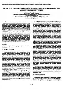
IV. SIMULATION RESULTS To demonstrate the performance of the proposed method, we compared it with the method of Wax and Ziskind [ 171 in several simulated experiments. In all the experiments the sources had equal power and impinged on a uniform and linear array with isotropic sensors spaced half a wavelength apart. The signals and the noise were distributed according to the SS and WN models, respectively. We performed 100 Monte Carlo runs and computed the relative frequency that the MDL criterion correctly detected the two sources as a function of the number of samples. We did that both for the proposed method, referred to as stochastic signals (SS), and for the method of Wax and Ziskind [ 171, referred to as deterministic signals (DS). We also computed the standard deviation (STD) of the estimators of the locations for the SS and DS methods. The SS estimators were computed by the alternating maximization (AM) technique [ 191, while the DS estimators were computed by the alternating projection (AP) technique [ 191, which is a variant of the alternating maximization technique. Both techniques transform the multidimensional optimization problem into a sequence of much simpler one-dimensional optimization problems that are iterated till convergence, and have a simple and efficient initialization. In the first experiment the sources were uncorrelated and impinged from 0" and 10". The number of sensors p was 3 and the signal-to-noise ratio was 0 dB. The results are shown in Fig. 1 . In the second experiment the sources were also uncorrelated but this time they impinged from 0" and 5 " . The number of sensors was 6 and the signal-to-noise ratio was 0 dB. The results are presented in Fig. 2.
24--
200
' 250
_ _ 300
I 350
500
M
(b) Fig. 1. Two equal power uncorrelated sources, located at 0" and IO", impinging on a linear uniform array with three sensors spaced half a wavelength apart. The SNR is 0 dB. (a) Probability of correct detection of the proposed method (SS) and the method of Wax and Ziskind (DS) as a function of the number of samples. (b) The standard deviation of the estimated location of the first source obtained by the estimator of the proposed method (SS) and the estimator of the method of Wax and Ziskind (DS), together with the Cramer-Rao bound (CR), as a function of the number of samples.
The results of the first two experiments demonstrate the improved performance of the proposed method over that of Wax and Ziskind. The gain in performance is especially notable in the threshold region. Not surprisingly, this gain is larger in the second experiment since in this case the difference between the number of free parameters between the two methods, given by 2(2p - k + 1) - (k - k 2 ) ,is larger. The results also demonstrate that the performance of estimators is essentially the same for the case of uncorrelated signals. In the third experiment, the scenario was the same as in the second experiment, except that in this case the two sources were coherent with phase difference of 90" at the array center. The results are presented in Fig. 3. This experiment demonstrates that the gain in the detection performance is greater in the case of coherent signals. It also demonstrates that the performance of the SS estimator outperforms the DS estimator, but that the gain in performance is marginal.
2455
WAX: DETECTION AND LOCALIZATION OF MULTIPLE SOURCES
Fig. 2 . Two equal power uncorrelated sources, located at 0" and 5 " , impinging on a linear uniform array with six sensors spaced half a wavelength apart. The SNR is 0 dB. (a) Probability of correct detection of the proposed method (SS) and the method of Wax and Ziskind (DS) as a function of the number of samples. (b) The standard deviation of the estimated location of the first source obtained by the estimator of the proposed method (SS) and the estimator of the method of Wax and Ziskind (DS), together with the Cramer-Rao bound (CR), as a function of the number of samples.
J 4,
6
P
~-~~-
- L
(a)
(b)
Fig 3 Two equal power coherent sources, located at 0" and 5". impinging on a linear uniform array with S I X sensors spaced half a wavelength apart The SNR is 0 dB and the phase difference at the array center is 90" (a) Probability of correct detection of the proposed method (SS) and the method of Wax and Ziskind (DS) as a function of the number of samples (b) The standard deviation of the estimated location of the first qource obtained by the estimator of the proposed method ( S S ) and the estimator of the method of Wax and Ziskind (DS) as a function of the number of samples
In all the experients, the number of iterations of the AM algorithm almost never exceeded 7, with the average being between 4 and 5. In fact, the convergence behavior was essentially identical to that of the AP algorithm. Finally, when the detection criteria failed in the above experiments, they almost always underestimated the number of sources.
V . CONCLUSIONS We have presented a novel solution to the detection of multiple sources which outperforms the recently proposed method of Wax and Ziskind [17]. The key to the improved performance is the small number of parameters characterizing the stochastic signals
model. In contrast to the method of Wax and Ziskind, in which the number of free parameters is p ( 2 p - q l), where q is the number of sources and p the number of sensors, in the proposed solution this number is given by q 2 q, which is always smaller since p > q. Another important factor in the improved performance is the maximum likelihood estimator for the stochastic signals model. In contrast to the maximum likelihood estimator of the deterministic signals used in the solution of Wax and Ziskind, which is inefficient, especially in the case of coherent signals, the maximum likelihood estimator of the stochastic signals model is efficient. The computational complexity of this method is similar to that of Wax and Ziskind [17] since both involve multidimensional minimization.
+
+
IEEE TRANSACTIONS ON SIGNAL PROCESSING. VOL. 39. NO. I I . NOVEMBER 1991
2456
APPENDIX CONSISTENCY OF THEML ESTIMATOR In this Appendix we prove the consistency of the ML estimator. Though this can be done by verifying that the ML estimator consistency conditions apply, we take a direct and more insightful approach using the form of the ML estimator given by ( 1 8). From ( 5 ) , suppressing the index k , we get
where bss(8) and respectively, and
bNN(8) are given 1
by (15.b) and (10.b),
M
&,(e) = M i C xs(ti)x;(tj). =(
(A1.b)
-
Taking the determinant of both sides, recalling that G ( 8 ) is unitary, we get
=
I &de> I I &de) &v(e> &.(0) &s(e) I -
(A2)
which, since ksN(8) &&e)&(e) is nonnegative definite, implies that
I I
5
I f i N d 0 ) I I &(e>I .
(‘43)
Now I1-Y
IffNde)l=
II r ( e >
(‘44)
r=l
and by (30)
(-
162(8)Z( = p
1 -
P-4
q
r=l
P-q
.!:(O,)
(A5)
where /:(e) 2 * * . 2 l:pq(8)denote the nonzero eigenvalues of the rank-@ - q) matrix P,&)kf‘,&). By the inequality of the arithmetic and geometric means we have 1 P-q 1lp-q (A6) p - q I = I fr(8)2 !:(e))
(:cy
with equality if and only if !:(e)= Hence, using (A4) and (A5), we obtain
I ffNd@)I
5
.
=
f/.N_&f3).
I 62(e)z1
ACKNOWLEDGMENT The author would like to thank D. Hertz and the reviewers for their careful reading of the paper and their helpful comments.
REFERENCES H. Akaike, “Information theory and an extension of the maximum likelihood principle,” in Proc. 2nd In/. Symp. Inform. Theory, B. N . Petrov and F. Caski, Eds. 1973, pp. 267-281. J . F. Bohme, “Estimation of spectral parameters of correlated signals in wavefields,” Signal Processing, vol. 1 I , pp. 329-337, 1986. J . E. Evans, J . R. Johnson, and D. F. Sun, “Application of advanced signal processing f angle-of-arrival estimation in ATC navigation and survilence systems.” M.I.T. Lincoln Lab., Lexington, MA, 1982, Rep. 582. A. G . Jaffer. “Maximum likelihood direction finding of stochastic sources: A separable solution,” in Proc. ICASSP 88, 1988, pp. 28932296. B. Ottersten and L. Ljung, “Asyptotic results for sensor array processing,” in Proc. lCASSP 89, 1989, pp. 2266-2269. J . Rissanen, “Modeling by the shortest data descrption,” Auromurim. vol. 14, pp. 465-471, 1978. J. Rissanen, “A universal prior for the integers and estimation by minimum description length,” Ann. Stat., vol. 1 1 . pp. 416-431, 1983. T. J . Shan, M . Wax, and T. Kailath. “On spatial smoothing for direction-of-arrival estimation of coherent sources,” IEEE Trans. 4coust.. Speech, Signal Processing, vol. 33, no. 4 , pp. 806-81 I , 1985. K . S h a m a n , “Maximum likelihood estimation by simulated annealing.” in Proc. lCASSP 88, 1988, pp. 2741-2744. K. S h a m a n and G . D. McClurkin, “Genetic algorithms for maximum likelihood parameter estimation,” in Proc. lCASSP 89, pp. 2716-2719. P. Stoica and A. Nehorai, “MUSIC, maximum likelihood, and the Cramer-Rao bound.” lEEE Truns. Acoust. , Speech, Signal Processing. vol. 37. pp. 720-743, 1989. P. Stoica and A. Nehorai, “MUSIC, maximum likelihood, and the Cramer-Rao bound: Further results and comparisons,” in Proc. lCASSP 8Y. 1989. H . Wang and M. Kaveh, ”Coherent signal-subspace processing for the detection and estimation of angles of arrival of multiple wide-band sources.” lEEE Truns. Acoust.. Speech, Signal Processing, vol. 33, no. 4, pp. 823-831. 1985. M. Wax, “Detection and estimation of superimposed signals,” Ph.D. dissertation. Stanford University, 1985. M . Wax and T . Kailath. “Detection of signals by information theoretic criteria.” IEEE Trans. Acoust., Speech, Signal Processing, vol. 33, pp. 387-392, 1985. M. Wax and I . Ziskind, “On unique localization of multiple sources in passive sensor arrays,” lEEE Trans. Acoust., Speech. Signal Processing. vol. 37, no. 7. pp. 996-1000, 1989. M. Wax and 1. Ziskind, “Detection of the number of coherent and noncoherent signals by the MDL principle.” IEEE Trans. Acoust., Speech. Signal Processing. vol. 37, no. 8, pp. 1190-1 196, 1989. L. C . Zhao, P. R. Krishnaiah, and Z . D. Bai, “On detection of the number of signals in the presence of white noise,” .I.Mulrivariafe Anul., vol. 20, pp. 1-20, 1986. 1. Ziskind and M. Wax, “Maximum likelihood localization of multiple sources by alternating projection,” IEEE Trans. Acoust., Speech, Signul Processing, vol. 36, pp. 1553-1560, 1988.
(‘47) Mati Wax (S’81-M’84-SM’88)
and therefore, by (A3),
I ~ 5 I I&(S)I I C2(e)zi with equality if and only if =
i;-q(e).
&,,(e)= 0 and .!:(e)=
(-48) *
*
Since both conditions are satisfied for the true 8 as M ---t 03, it follows that the minimum of (18) in the case of M 03 is obtained at the true 8 . This establishes the consistency of the ML estimator 6. -+
received the B.Sc. and M.Sc. degrees from the Technion, Haifa, Israel, in 1969 and 1975, respectively. and the Ph.D. degree from Stanford University, Stanford, CA, in 1985, all in electrical engineering. From 1969 to 1973 he served as an Electronic Engineer in the Israeli Army. In 1974 he was with A.E.L., Israel. In 1975 he joined RAFAEL, where he is currently heading the Center for Signal Processing. In 1984 he was a Visiting Scientist at IBM Research Laboratories, San Jose, CA. His research interests are in signal processing and statistical modeling. Dr. Wax was the recipient of the 1985 Senior Paper Award of the IEEE T R A N S A C T I O N S OY ACOUSTICS. SPEF,CH, A N D SIGNAL PROCESSING.