On Universal Search Strategies for Multi-Criteria Optimization Using ...

On Universal Search Strategies for Multi-Criteria Optimization Using Weighted Sums Julien Legriel, Scott Cotton and Oded Maler CNRS-Verimag 2 av. de Vignate, 38610 Gieres, FRANCE Email: {legriel,cotton,maler}@imag.fr

Abstract—We develop a stochastic local search algorithm for finding Pareto points for multi-criteria optimization problems. The algorithm alternates between different single-criterium optimization problems characterized by weight vectors. The policy for switching between different weights is an adaptation of the universal restart strategy defined by [LSZ93] in the context of Las Vegas algorithms. We demonstrate the effectiveness of our algorithm on multi-criteria quadratic assignment problem benchmarks and prove some of its theoretical properties.

I. I NTRODUCTION The design of complex systems involves numerous optimization problems, where design choices are encoded as valuations of decision variables and the relative merits of each choice are expressed via a utility/cost function over these variables. In many real-life situations one has to deal with cost functions which are multi-dimensional. For example, a cellular phone that we want to purchase or develop can be evaluated according to its cost, screen size, power consumption and performance. A configuration s which dominates s0 according to one criterium, can be worse according to another. In the absence of a linear ordering of the alternatives, there is no unique optimal solution but rather a set of efficient solutions, also known as Pareto solutions [Par12]. Such solutions are characterized by the property that their cost cannot be improved in one dimension without being worsened in another. The set of all Pareto solutions, the Pareto front, represents the problem trade-offs, and being able to sample this set in a representative manner is a very useful aid in decision making. In this paper we study the adaptation of stochastic local search (SLS) algorithms, used extensively in (singleobjective) optimization and constraint satisfaction problems, to the multi-objective setting. SLS algorithms perform a guided probabilistic exploration of the decision space where at each time instance, a successor is selected among the neighbors of a given point, with higher probability for locally-optimal points. SLS algorithms can be occasionally restarted, where restart means abandoning the current point and starting from scratch. It has been observed (and proved) [LSZ93] that in the absence of a priori knowledge about the cost landscape, scheduling such restarts according to a specific pattern boosts the performance of such algorithm in terms of expected time to find a solution. This has led to successful algorithms for several problems, including SAT [PD07].

One popular approach for handling multi-objective problems is based on optimizing a one-dimensional cost function defined as a weighted sum of the individual costs according to a weight vector λ. Repeating the process with different values of λ leads to a good approximation of the Pareto front. Our major contribution is an algorithmic scheme for distributing the optimization effort among different values of λ. To this end we adapt the ideas of [LSZ93] to the multi-objective setting and obtain an algorithm which is very efficient in practice. The rest of this paper is organized as follows. In Section II we introduce an abstract view of randomized optimizers and recall the problematics of multi-criteria optimization. Section III discusses the role of restarts in randomized optimization. Section IV presents our algorithm and proves its properties. Section V provides experimental results and Section VI concludes. II. BACKGROUND A. SLS Optimization Randomization has long been a useful tool in optimization. In this paper, we are concerned with optimization over finite domain functions by means of stochastic local search (SLS) [HS04], in the style of such tools as WalkSAT [SKC96], UBCSAT [TH04] or LKH [Hel09]. Here we provide a simplified overview in which we consider only a minimal characterization of SLS necessary for the paper as a whole. We assume a finite set X called the decision space whose elements are called points. We assume some metric ρ on X which in a combinatorial setting corresponds to a kind of Hamming distance where ρ(s, s0 ) characterizes the number of modifications needed to transform s to s0 . The neighborhood of s is the set N (s) = {s0 : ρ(s, s0 ) = 1}. A cost (objective) function f : X → R is defined over X and is the subject of the optimization effort. We call the range of f the cost space and say that a cost o is feasible if there is s ∈ X such that f (s) = o. A random walk is a process which explores X starting from an initial randomly-chosen point s by repeatedly stepping from s to a neighboring point s0 , computing f (s0 ) and storing the best point visited so far. In each step, the next point s0 is selected according to some probability distribution Ds over X which we assume to be specific to point s. Typically, Ds gives non-zero probability to a small portion of X included in N (s).

While the particular probability distributions vary a great deal such processes, including [SKC96], [TH04], [Hel09], also share many properties. Some such properties are crucial to the performance of SLS optimization algorithms. For example, all processes we are aware of favor local optima in the probability distributions from which next states are selected. The efficiency of such processes depends on structural features of the the decision space such as the size of a typical neighborhood and the maximal distance between any pair of points, as well as on the cost landscape. In particular, cost landscapes admitting vast quantities of local optima and very few global optima and where the distances between local and global optima are high, tend to be difficult for random walk algorithms [HS04, Ch. 5]. Of particular interest to this paper, a simple and common practice exploited by SLS based optimization tools is restarting. In our simplified model of random walk processes, a restart simply chooses a next state as a sample from a constant initial probability distribution rather than the nextstate probability distribution. Typically the process may start over from a randomly generated solution or from a constant one which has been computed off-line. Restarting can be an effective means for combating problematics associated with the cost landscape. It is particularly efficient in avoiding stagnation of the algorithm and escaping a region with local optima. Most search methods feature a mechanism to thwart this behavior, but this might be insufficient sometimes. For instance a tabu search process may be trapped inside a long cycle that it fails to detect. Another aspect in which restarts may help is to limit the influence of the random number generator. Random choices partly determine the quality of the output and starting from scratch is a fast way to cancel bad random decisions that were made earlier. As we will argue, restarting can also be effectively exploited for multi-criteria problems. B. Multi-criteria Optimization Multi-criteria optimization problems seek to optimize a multi-valued objective f : X → Rd which we can think of as a vector of costs (f 1 , . . . , f d ). When d > 1 the cost space is not linearly-ordered and there is typically no single optimal point, but rather a set of efficient points known as the Pareto front, consisting of non-dominated feasible costs. We recall some basic vocabulary related to multi-objective optimization. The reader is referred to [Ehr05], [Deb01] for a general introduction to the topic. Definition 1 (Domination): Let o and o0 be points in the cost space. We say that o dominates o0 , written o @ o0 , if for every i ∈ [1..d], oi ≤ o0i and o 6= o0 . Definition 2 (Pareto Front): The Pareto front associated with a multi-objective optimization problem is the set O∗ consisting of all feasible costs which are not dominated by other feasible costs. A popular approach to tackle multi-objective optimization problems is to reduce them to several single-objective ones.

Definition 3 (λ-Aggregation): Let f = (f 1 , . . . , f d ) be a d-dimensional function and let λ = (λ1 , . . . , λd ) be a vector such that 1) P ∀j ∈ [1..d], λj > 0 d j 2) j=1 λ = 1; and The λ-aggregation of f is the function fλ =

d X

λj f j .

j=1

Intuitively, the components of λ represent the relative importance (weight) one associates with each objective. A point which is optimal with respect to fλ is also a Pareto point for the original cost function. Conversely, when the Pareto front is convex in the cost space, every Pareto solution corresponds to an optimal point for some f λ . At this point it is also important to explain why we choose to optimize weighted sums of the objectives while being aware of one major drawback of this technique: the theoretical impossibility to reach Pareto points on concave parts of the front. Actually negative results [Ehr05] only state that some solutions are not optimal under any combination of the objectives, but we may nevertheless encounter them while making steps in the decision space. This fact was also confirmed experimentally (see Section V-A), as we found the whole non-convex Pareto front for small instances where it is known. C. Related Work Stochastic local search methods are used extensively for solving hard combinatorial optimization problems for which exact methods do not scale [HS04]. Among the well known techniques we find simulated annealing [KGV83], tabu search [GM06], ant colony optimization [CDM92] and evolutionary algorithms [Mit98], [Deb01] each of which has been applied to hard combinatorial optimization problems such as the traveling salesman, scheduling or assignment problems. Many state-of-the-art local search algorithms have their multi-objective version [PS06]. For instance, there exists multi-objective extensions of simulated annealing [CJ98], [BSMD08] and tabu search [GMF97]. A typical way of treating several objectives in that context is to optimize a predefined or dynamically updated series of linear combinations of the cost functions. A possible option is to pick a representative set of weight vectors a priori and run the algorithm for each scalarization successively. This has been done in [UTFT99] using simulated annealing as a backbone. More sophisticated methods have also emerged where the runs are made in parallel and the weight vector is adjusted during the search [CJ98], [Han97] in order to improve the diversity of the population. Weight vectors are thus modified such that the different runs are guided towards distinct unexplored parts of the cost space. One of the main issues in using the weighted sum method is therefore to share the time between different promising search directions (weight vectors) appropriately. Generally deterministic strategies are used: weight vectors are predetermined, and they may be modified dynamically according to a deterministic heuristic. However, unless some knowledge on the cost space

has been previously acquired, one may only speculate on the directions which are worth exploring. This is why we study in this work a completely stochastic approach, starting from the assumption that all search directions are equally likely to improve the final result. The goal we seek is therefore to come up with a scheme ensuring a fair time sharing between different weight vectors. Also related to this work are population-based genetic algorithms which naturally handle several objectives as they work on several individual solutions that are mutated and recombined. They are vastly used due to their wide applicability and good performance and at the same time they also benefit from combination with specialized local search algorithms. Indeed some of the top performing algorithms for solving combinatorial problems are hybrid, in the sense that they mix evolutionary principles with local search. This led to the class of so called memetic algorithms [KC05]. It is common that scalarizations of the objectives are used inside such algorithms for guiding the search, and choosing a good scheme to adapt weight vectors dynamically is also an interesting issue. The work presented in this paper began while trying to combine two ingredients used for solving combinatorial problems: the above mentioned scalarization of the objectives and restarts. Restarts have been used extensively in stochastic local search since they usually bring a significant improvement in the results. For instance greedy randomized adaptive search procedures (GRASP) [FR95] or iterated local search [LMS03] are well-known methods which run successive local search processes starting from different initial solutions. In [HS04, Ch. 4] restarts in the context of single-criteria SLS are studied. Their technique is based on an empirical evaluation of runtime distributions for some classes of problems. In this work, we devise multi-criteria restarting strategies which perform reasonably well no matter what the problem or structure of the cost space happens to be. The main novelty is a formalization of the notion of a universal multi-criteria restart strategy: every restart is coupled with a change in the direction and restarts are scheduled to balance the effort across directions and run times. This is achieved by adapting the ideas of [LSZ93], presented in the next section, to the multi-objective setting. III. R ESTARTING S INGLE C RITERIA SLS O PTIMIZERS This practice of restarting in SLS optimization has been in use at least since [SKC96]. At the same time, there is a theory of restarts formulated in [LSZ93] which applies to Las Vegas algorithms which are defined for decision problems rather than optimization. Such algorithms are characterized by the fact that their run time until giving a correct answer to the decision problem is a random variable. In the following we recall the results of [LSZ93] and analyze their applicability to optimization using SLS. We begin by defining properly what a strategy for restarting is. Definition 4 (Restart Strategy): A restart strategy S is an infinite sequence of positive integers t1 , t2 , t3 , . . .. The t time prefix of a restart strategy S, denoted S[t] is the maximal sequence t1 , . . . , tk such that Σki=1 ti ≤ t.

Running a Las Vegas algorithm according to strategy S means running it for t1 units of time, restarting it and running it for t2 units of time and so on. A. The Luby Strategy A strategy is called constantly repeating if it takes the form c, c, c, c, . . . for some positive integer c. As shown in [LSZ93] every Las Vegas algorithm admits an optimal restart strategy which is constantly repeating (the case of infinite c is interpreted as no restarting). However, this fact is not of much use because typically one has no clue for finding the right c. For these reasons, [LSZ93] introduced the idea of universal strategies that “efficiently simulate” every constantly repeating strategy. To get the intuition for this notion of simulation and its efficiency consider first the periodic strategy S = c, c0 , c, c0 , c, c0 , . . . with c < c0 . Since restarts are considered independent, following this strategy for m(c + c0 ) steps amounts to spending mc time according to the constant strategy c and mc0 time according to strategy c0 .1 Putting it the other way round, we can say that in order to achieve (expected) performance as good as running strategy c0 for t time, it is sufficient to run S for time t + c(t/c0 ). The function f (t) = t+c(t/c0 ) is the delay associated with the simulation of c0 by S.2 It is natural to assume that a strategy which simulates numerous other strategies (i.e has sub-sequences that fit each of the simulated strategies) admits some positive delay. Definition 5 (Delay Function): A monotonic non decreasing function δ : N → N, satisfying δ(x) ≥ x is called a delay function. We say that S simulates S 0 with delay bounded by δ if running S 0 for t time is not better than running S for δ(t) time. It turns out that a fairly simple strategy, which has become known as the Luby strategy, is universally efficient. Definition 6 (The Luby Strategy): The Luby Strategy is the sequence c1 , c2 , c3 , . . . where . ci =



2k−1 ti−2k−1 +1

if i = 2k − 1 if 2k−1 ≤ i < 2k − 1

which gives 1, 1, 2, 1, 1, 2, 4, 1, 1, 2, 1, 1, 2, 4, 8, . . .

(1)

We denote this strategy by L. A key property of this strategy is that it naturally multiplexes different constant strategies. For instance the prefix 1 contains eight 10 s, four 20 s, two 40 s and one 8, and the total times dedicated to strategies 1, 2, 4 and 8 are equal. More formally, let A(c) denote the fact that a Las Vegas algorithm A is run with constant restart c. Then, the sum of the execution times 1 In fact, since running an SLS process for c0 is at least as good as running it for c time, running S for m(c + c0 ) is at least as good as running c for m(c + c) time. 2 For simplicity here we consider the definition of the delay only at time instants t = kc0 , k ∈ N. In the case where t = kc0 + x, where x is an integer such that 0 < x < c0 , the delay function would be δ(t) = bt/c0 cc + t.

spent on A(2i ) is equal for all 1 ≤ i < 2k−1 over a 2k − 1 length prefix of the series. As a result, every constant restart strategy where the constant is a power of 2 is given an equal time budget. This can also be phrased in terms of delay. Proposition 1 (Delay of L ): Strategy L simulates any strategy c = 2a with delay δ(t) ≤ t(blog tc + 1). Sketch of proof: Consider a constant strategy c = 2a and a time t = kc, k ∈ N. At the moment where the k th value of c appears in L, the previous ones in the sequence are all of the form 2i for some i ∈ {0..blog tc}. This is because the series is built such that time is doubled before any new power of two is introduced. Furthermore after the execution of the k th c, every 2i constant with i ≤ a has been run for exactly t time, and every 2i constant with i > a (if it exists in the prefix) has been executed less than t time. This leads to δ(t) ≤ t(blog tc + 1). This property implies that restarting according to L incurs a logarithmic delay over using the unknown optimal constant restart strategy of a particular problem instance. Additionally the strategy is optimal in the sense that it is not possible to have better than logarithmic delay if we seek to design a strategy simulating all constant restart strategies [LSZ93]. The next section investigates how these fundamental results can be useful in the context of optimization using stochastic local search.

distributions one could decide which o is more likely to be found before t and invest more time for the associated optimal constant restart strategies. But without that knowledge every constant restart strategy might be useful for converging to a good approximation of o∗ . Therefore whereas Las Vegas algorithms run different constant restart strategies because it is impossible to know the optimal c∗ , an SLS process runs them because it does not know which approximation o is reachable within a fixed time t, and every such o might be associated with a different optimal constant restart strategy. This remark further motivates the use of strategy L for restarting an SLS optimizer. IV. M ULTI - CRITERIA S TRATEGIES In this section we extend strategy L to become a multicriteria strategy, that is, a restart strategy which specifies what combinations of criteria to optimize and for how long. We assume throughout a d-dimensional cost function f = (f 1 , . . . , f d ) convertible into a one-dimensional function fλ associated with a weight vector λ ranging over a bounded set Λ of a total volume V . Definition 8 (Multi-criteria Strategy): A multi-criteria search strategy is an infinite sequence of pairs S = (t(1), λ(1)), (t(2), λ(2)), . . .

An SLS optimizer is an algorithm whose run-time distribution for finding a particular cost o is a random-variable. Definition 7 (Expected Time): Given an SLS process and a cost o, the random variable Θo indicates the time until the algorithm outputs a value at least as good as o. There are some informal reasons suggesting that using strategy L in the context of optimization would boost the performance. First, a straightforward extension of results of Section III-A to SLS optimizers can be made. Corollary 1: Restarting an SLS process according to strategy L gives minimum expected run-time to reach any cost o for which Θo is unknown. The corollary follows directly because the program that runs the SLS process and stops when the cost is at least as good as o is a Las Vegas algorithm whose run-time distribution is Θo . In particular, using strategy L in that context gives a minimal expected time to reach the optimum o∗ . Still, finding the optimum is too ambitious for many problems and in general we would like to run the process for a fixed time t and obtain the best approximation possible within that time. A priori there is no reason for which minimizing the expected time to reach the optimum would also maximize the approximation quality at a particular time t. On the contrary, for each value of o we have more or less chances to find a cost at least as good as o within time t depending on the probability P (Θo ≤ t).3 Knowing the

where for every i, t(i) is a positive integer and λ(i) ∈ Λ is a weight vector. The intended meaning of such a strategy is to run an SLS process to optimize fλ(1) for t(1) steps, then fλ(2) for t(2) and so on. Following such a strategy and maintaining the set of non-dominated solutions encountered along the way yields an approximation of the Pareto front of f . Had Λ been a finite set, one could easily adapt the notion of simulation from the previous section and devise a strategy which simulates with a reasonable delay any constant strategy (λ, c) for any λ ∈ Λ. However since Λ is infinite we need a notion of approximation. Looking at two optimization processes, one for fλ and one for fλ0 where λ and λ0 are close to each other, we observe that the functions may not be very different and the effort spent in optimizing fλ is almost in the same direction as optimizing fλ0 . This motivates the following definition. Definition 9 (-Approximation): A strategy S -approximates a strategy S 0 if for every i, t(i) = t0 (i) and |λ(i) − λ0 (i)| < . From now on we are interested in finding a strategy which simulates with good delay an -approximation of any constant strategy (λ, c). To build such an -universal strategy we construct an -net D for Λ, that is, a minimal subset of Λ such that for every λ ∈ Λ there is some µ ∈ D satisfying |λ − µ| < . In other words, D consists of representatives of all possible optimization directions. The cardinality of D depends on the metric used and we take it to be4 m = V (1/)d . Given D we can create a strategy which

3 Note that these probabilities are nondecreasing with o since the best cost value encountered can only improve over time.

4 Using other metrics the cardinality may be related to lower powers of 1/ but the dependence on  is at least linear.

B. SLS optimizers

is a cross product of L with D , essentially interleaving m instances of L. Clearly, every λ ∈ Λ will have at least 1/m of the elements in the sequence populated with -close values. Definition 10 (Strategy LD ): Let D be a finite subset of Λ admitting m elements. Strategy LD = (t(1), λ(1)), . . . is defined for every i as 1) λ(i) = λ(i mod m) 2) t(i) = L(d mi e) Proposition 2 (LD delay): Let D be an -net for Λ. Then LD simulates an -approximation of any constant strategy (λ, c) with delay δ(t) ≤ tm (blog tc + 1). Proof: For any constant (λ, c) there is an -close µ ∈ D which repeats every mth  time in LD . Hence the delay of LD with respect to L is at most m t and combined with the delay t(blog tc + 1) of L wrt any constant strategy we obtain the result. For a given , LD is optimal as the following result shows. Proposition 3 (LD Optimality): Any strategy that simulates every constant strategy has delay δ(t) ≥ m t/2(blog tc/2 + 1) with respect to each of those strategies. Proof Sketch: Consider such a multi-criteria strategy and t steps spent in that strategy. Let Si,j denote the multicriteria constant strategy (λi , 2j ), (λi , 2j ) . . . for all λi ∈ D and j ∈ {0, . . . , blog tc}. The minimum delay when simulating all Si,j for a fixed i is t/2(blog tc/2 + 1) (see the technical report [LCM11] for details). Because any two λi , λ0i ∈ D do not approximate each other, the delays for simulating constant strategies associated with different directions just accumulate. Hence δ(t) ≥ m t/2(blog tc/2 + 1). Despite these results, the algorithm has several drawbacks. First, computing and storing elements of an -net in high dimension is not straightforward. Secondly, multi-dimensional functions of different cost landscapes may require different values of  in order to explore their Pareto fronts effectively and such an  cannot be known in advance. In contrast, strategy LD needs a different D for each  with D growing as  decreases. In fact, the only strategy that can be universal for every  is a strategy where D is the set of all rational elements of Λ. While such a strategy can be written, its delay is, of course, unbounded. For this reason, we propose a stochastic restart strategy which, for any , -simulates all constant multi-criteria strategies with a good expected delay. Our stochastic strategy Lr is based on the fixed sequence of durations L and on random sequences of uniformly-drawn elements of Λ. Definition 11 (Strategy Lr ): • A stochastic multi-criteria strategy is a probability distribution over multi-criteria strategies; r • Stochastic strategy L generates strategies of the form (t(1), λ(1)), (t(2), λ(2)), . . . where t(1), t(2), . . . is L and each λ(i) is drawn uniformly from Λ.

Note that for any  and λ the probability of an element in the sequence to be -close to λ is 1/m . Let us try to give the intuition why for any  > 0 and constant strategy (λ, c), Lr probabilistically behaves as LD in the limit. Because each λ(i) is drawn uniformly, for any  > 0 the expected number of times λ(i) is -close to λ is the same for any λ ∈ Λ. So the time is equally shared for -simulating different directions. Moreover the same time is spent on each constant c as we make use of the time sequence L. Consequently Lr should simulate fairly every strategy (λ, c). We have not yet computed the expected delay5 with which a given multi-criteria strategy is simulated by Lr . Nonetheless a weaker reciprocal result directly follows: on a prefix of Lr of length tm (blog tc + log m +1), the expected amount of time -spent on any multicriteria constant strategy (λ, c) is t. Proposition 4 (Lr Expected Efficiency): for all  > 0, after a time T = tm (blog tc + log m + 1) in strategy Lr , the random variable wλ,c (T ) indicating the time spent on simulating any constant strategy (λ, c) verifies E[wλ,c (T )] = t. Proof: In time T , Lr executes tm times any constant c (proposition 1). On the other hand the expected fraction of that time spent for a particular λ is 1/m . V. E XPERIMENTS A. Quadratic Assignment Problem The quadratic assignment problem (QAP) is a hard unconstrained combinatorial optimization problem with many real-life applications related to the spatial layout of hospitals, factories or electrical circuits. An instance of the problem consists of n facilities whose mutual interaction is represented by an n × n matrix F with Fij characterizing the quantity of material flow from facility i to j. In addition there are n locations with mutual distances represented by an n × n matrix D. A solution is a bijection from facilities to locations whose cost corresponds to the total amount of operational work, which for every pair of facilities is the product of their flow with the distance between their respective locations. Viewing a solution as a permutation π on {1, . . . , n} the cost is formalized as n X n X C(π) = Fij · Dπ(i),π(j) . i=1 j=1

The problem is NP-complete, and even approximating the minimal cost within some constant factor is NP-hard [SG76]. 1) QAP SLS Design: We implemented an SLS-based solver for the QAP, as well as multi-criteria versions described in the preceding section. The search space for the solver on a problem of size n is the set of permutations of {1, .., n}. We take the neighborhood of a solution π to be the set of solutions π 0 that can be obtained by swapping two elements. This kind of move is quite common when solving QAP problems using local search. Our implementation also uses a standard incremental algorithm [Tai91] for maintaining the costs of all 5 It involves computing the expectation of the delay of L applied to a random variable with negative binomial distribution.

Algorithm 1 Greedy Randomized Local Search if rnd() ≥ p then optimal move() else rnd move() end if 2) Experimental Results on the QAP library: The QAP library [BKR97] is a standard set of benchmarks of one dimensional quadratic assignment problems. Each problem in the set comes with an optimal or best known value. We ran Algorithm 1 (implemented in C) using various constant restart strategies as well as strategy L on each of the 134 instances of the library.6 Within a time bound of 500 seconds per instance the algorithm finds the best known value for 93 out of 134 instances. On the remaining problems the average deviation from the optimum was 0.8%. Also the convergence is fast on small instances (n ≤ 20) as most of them are brought to optimality in less than 1 second of computation. Figure 1 plots for each strategy the number of problems brought to optimal or best-known values as a function of time. For a time budget of 500 seconds, strategy L was better than any constant strategy we tried. This fact corroborates the idea that strategy L is universal, in the sense that multiplexing several constant restart values makes it possible to solve (slightly) more instances. This is however done with some delay as observed in Figure 1 where strategy L is outperformed by big constant restarts (1024,10000,∞) when the total time budget is small. 6 The machine used for the experiments has an Intel Xeon 3.2GHz processor. Complete results of the simulations are not reported due to lack of space, but may be found in the technical report [LCM11].

90 num. best found

neighbors of the current point, which we briefly recall here. Given an initial point, we compute (in cubic time) and store the cost of all its neighbors. After swapping two elements (i, j) of the permutation, we compute the effect of swapping i with j on all costs in the neighborhood. Since we have stored the previous costs, adding the effect of a given swap to the cost of another swap gives a new cost which is valid under the new permutation. This incremental operation can be performed in amortized constant time for each swap, and there are quadratically many possible swaps, resulting in a quadratic algorithm for finding an optimal neighbor. Concerning the search method, we use a simple greedy selection randomized by noise (Algorithm 1). This algorithm is very simple but, as shown in the sequel, is quite competitive in practice. The selection mechanism works as follows: with probability 1 − p the algorithm makes an optimal step (ties between equivalent neighbors are broken at random), otherwise it goes to a randomly selected neighbor. Probability p can be set to adjust the noise during the search. Note that we have concentrated our effort on the comparison of different adaptive strategies for the weight vector rather than on the performance comparison of Algorithm 1 with the other classical local search methods (simulated annealing, tabu search).

80 c = 128 c = 256 c = 512 c = 1024 c = 10000 no restarts strategy L

70 60 50 0

100

200

300

400

500

time (sec) Fig. 1. Results of different restart strategies on the 134 QAPLIB problems with optimal or best known results available. Strategy L solves more instances than the constant restart strategies, supporting the idea that it is efficient in the absence of inside knowledge.

B. Multi-objective QAP The multi-objective QAP (mQAP), introduced in [KC03] admits multiple flow matrices F1 , . . . , Fd . Each pair (Fi , D) defines a cost function as presented in Section V-A, what renders the problem multi-objective. We have developed an extension of Algorithm 1 where multiple costs are agglomerated with weighted sums and the set of all non-dominated points encountered during the search is stored in an appropriate structure. In order to implement strategy Lr one also needs to generate d-dimensional random weight vectors which are uniformly distributed. Actually, generating random weight vectors is equivalent to sampling uniformly random points on a unit simplex, which is in turn equivalent to sampling from a Dirichlet distribution where every parameter is equal to one. The procedure for generating random weight vectors is therefore the following: 1. Generate d IID random samples (a1 , . . . , ad ) from a unit-exponential distribution, which is done by sampling ai from (0,1] uniformly and returning −log(ai ). 2. Normalize the P vector thus obtained by dividing d each coordinate by the sum i=0 ai . Multi-criteria strategies Lr and LD have been tested and compared on the benchmarks of the mQAP library, which includes 2-dimensional problems of size n = 10 and n = 20, and 3-dimensional problems of size n = 30 [KC03]. The library contains instances generated uniformly at random as well as instances generated according to flow and distance parameters which reflects the probability distributions found in real situations. Pre-computed Pareto sets are provided for all 10-facility instances. Note that our algorithm found over 99% of all Pareto points from all eight 10-facility problems within a total computation time of under 1 second.

1uni, strategy LD

1rl, constant restarts 1 0.99 0.95 Lr c = 10 c = 100 c = 1000

0.9 0

20

40

0.98

Lr  = 0.1  = 0.01  = 0.001

0.97

60

0

20

40

time (sec)

time (sec)

1uni, constant restarts

1rl, strategy LD

60

1 0.99

0.98

0.98

0.96 Lr c = 10 c = 100 c = 1000

0.97 0.96 0

20

40

60

time (sec) Fig. 2. Performance of various constant multi-criteria strategies against Lr on the 1rl and 1uni 20-facility problems. The metric used is the normalized epsilon indicator, the reference set being the union of all solutions found. In these experiments constant restarts values c = 10, 100, 1000 are combined with randomly generated directions.

For the remaining problems where the actual Pareto set is unknown, we resort to comparing performance against the non-dominated union of solutions found with any configuration. As a quality metric we use the epsilon indicator [ZKT08] which is the largest increase in cost of a solution in the reference set, when compared to its best approximation in the set to evaluate. The errors are normalized with respect to the difference between the maximal and minimal costs in each dimension over all samples of restart strategies leading to a number α ∈ [0, 1] indicating the error with respect to the set of all found solutions.7 Figures 2, 3 and 4 depict the results of the multi-criteria experiments. We compared Lr against constant restarts combined with randomly chosen directions and strategy LD for different values of . Despite its theoretical properties LD does not perform so good for the  values that we chose. This corroborates the fact that it is hard to guess a good  value beforehand. Constant restarting works well but the appropriate constant has to be carefully chosen. At the end strategy Lr gives decidedly better performance amongst all 7 In the future we also intend to use techniques which can formally validate a bound on the quality of a Pareto set approximation [LGCM10] in order to assess the efficiency of this algorithm.

Lr  = 0.1  = 0.01  = 0.001

0.94 0.92 0

20

40

60

time (sec) Fig. 3. Performance of LD multi-criteria strategies against Lr on the 1rl and 1uni 20-facility problems for  = 0.1, 0.01, 0.001.

the strategies we tried. It is worth noting that we also tried using the weighted infinity norm maxi λi f i as a measure of cost but, despite its theoretical superiority (any Pareto point on a concave part of the front is optimal for some λ), the method did perform worse than the weighted sum approach in our experiments. VI. C ONCLUSION We have demonstrated how efficient universal strategies can accelerate SLS-based optimization, at least in the absence of knowledge of good restart constants. In the multi-criteria setting our universal strategy is efficient, both theoretically and experimentally and gives a thorough and balanced coverage of the Pareto front. Having demonstrated the strength of our algorithm on the QAP benchmarks, we are now working on two extensions of this work. First, we are planning to use strategy Lr with other efficient local search techniques, starting with tabu search [Tai91]. Secondly we intend to move on to problems associated with mapping and scheduling of programs on multi-processor architectures and see how useful this algorithmics can be for those problems.

KC30-3fl-2uni

[HS04]

·106 2.1 c3

2 1.9

1.9

2 1.9

2

c1

·106

c2 ·106 KC30-3fl-2rl

c3

·107 2 1 3 4

c1

0.6

0.8

7

·10

c2

1 ·107

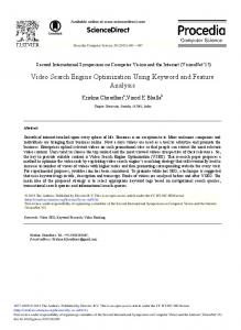
Fig. 4. Examples of approximations of the Pareto front for two 30-facility, 3flow QAP problems. KC30-3fl-2uni was generated uniformly at random while KC30-3fl-2rl was generated at random with distribution parameters, such as variance, set to reflect real problems. The approximations above are a result of 1 minute of computation using Lr as multi-criteria strategy.

R EFERENCES [BKR97]

R.E. Burkard, S.E. Karish, and F. Rendl. QAPLIB – a quadratic assignment problem library. Journal of Global Optimization, 10:391–403, 1997. [BSMD08] S. Bandyopadhyay, S. Saha, U. Maulik, and K. Deb. A simulated annealing-based multiobjective optimization algorithm: AMOSA. IEEE Transactions on Evolutionary Computation, 12(3):269– 283, 2008. [CDM92] A. Colorni, M. Dorigo, and V. Maniezzo. Distributed optimization by ant colonies. In Proceedings of the first European conference on artificial life, pages 134–142, 1992. [CJ98] P. Czyzak and A. Jaszkiewicz. Pareto simulated annealing - a metaheuristic technique for multiple-objective combinatorial optimization. Journal of Multi-Criteria Decision Analysis, 7(1):34– 47, 1998. [Deb01] K. Deb. Multi-objective optimization using evolutionary algorithms. Wiley, 2001. [Ehr05] M. Ehrgott. Multicriteria optimization. Springer Verlag, 2005. [FR95] T.A. Feo and M.G.C. Resende. Greedy randomized adaptive search procedures. Journal of Global Optimization, 6(2):109– 133, 1995. [GM06] F. Glover and R. Marti. Tabu search. Metaheuristic Procedures for Training Neutral Networks, pages 53–69, 2006. [GMF97] X. Gandibleux, N. Mezdaoui, and A. Fr´eville. A tabu search procedure to solve multiobjective combinatorial optimization problem. Lecture notes in economics and mathematical systems, pages 291–300, 1997. [Han97] M.P. Hansen. Tabu search for multiobjective optimization: MOTS. In Proc. 13th Int. Conf on Multiple Criteria Decision Making (MCDM), pages 574–586, 1997. [Hel09] K. Helsgaun. General k-opt submoves for the Lin-Kernighan TSP heuristic. Mathematical Programming Computation, 2009.

H. Hoos and T. St¨utzle. Stochastic Local Search: Foundations and Applications. Morgan Kaufmann / Elsevier, 2004. [KC03] J. Knowles and D. Corne. Instance generators and test suites for the multiobjective quadratic assignment problem. In EMO, volume 2632 of LNCS, pages 295–310. Springer, 2003. [KC05] J. Knowles and D. Corne. Memetic algorithms for multiobjective optimization: issues, methods and prospects. Recent advances in memetic algorithms, pages 313–352, 2005. [KGV83] S. Kirkpatrick, C. D. Gelatt, and M. P. Vecchi. Optimization by simulated annealing. Science, 220 (4598):671–680, 1983. [LCM11] J. Legriel, S. Cotton, and O. Maler. On universal search strategies for multi-criteria optimization using weighted sums. Technical Report TR-2011-7, Verimag, 2011. [LGCM10] J. Legriel, C. Le Guernic, S. Cotton, and O. Maler. Approximating the Pareto front of multi-criteria optimization problems. In TACAS, volume 6015 of LNCS, pages 69–83. Springer, 2010. [LMS03] H. Lourenco, O. Martin, and T. St¨utzle. Iterated local search. Handbook of metaheuristics, pages 320–353, 2003. [LSZ93] M. Luby, A. Sinclair, and D. Zuckerman. Optimal speedup of Las Vegas algorithms. In Israel Symposium on Theory of Computing Systems, pages 128–133, 1993. [Mit98] M. Mitchell. An introduction to genetic algorithms. The MIT press, 1998. [Par12] V. Pareto. Manuel d’´economie politique. Bull. Amer. Math. Soc., 18:462–474, 1912. [PD07] K. Pipatsrisawat and A. Darwiche. A lightweight component caching scheme for satisfiability solvers. In SAT, volume 4501 of LNCS, pages 294–299. Springer, 2007. [PS06] L. Paquete and T. St¨utzle. Stochastic local search algorithms for multiobjective combinatorial optimization: A review. Technical Report TR/IRIDIA/2006-001, IRIDIA, 2006. [SG76] S. Sahni and T. Gonzalez. P-complete approximation problems. Journal of the ACM, 23:555–565, 1976. [SKC96] B. Selman, H.A. Kautz, and B. Cohen. Local search strategies for satisfiability testing. In DIMACS Series in Discrete Mathematics and Theoretical Computer Science, 1996. [Tai91] E. Taillard. Robust taboo search for the quadratic assignment problem. Parallel computing, 17(4-5):443–455, 1991. [TH04] D. Tompkins and H. Hoos. UBCSAT: An implementation and experimentation environment for SLS algorithms for SAT & MAX-SAT. In SAT, volume 3542 of LNCS, pages 306–320. Springer, 2004. [UTFT99] E.L. Ulungu, J. Teghem, P.H. Fortemps, and D. Tuyttens. MOSA method: a tool for solving multiobjective combinatorial optimization problems. Journal of Multi-Criteria Decision Analysis, 8(4):221–236, 1999. [ZKT08] E. Zitzler, J. Knowles, and L. Thiele. Quality assessment of pareto set approximations. In Multiobjective Optimization, volume 5252 of LNCS, pages 373–404. Springer, 2008.