ON VALIDATING DESIGN DECISION METHODOLOGIES

Proceedings of DETC 2003 ASME 2003 Design Engineering Technical Conferences Design Theory and Methodology Conference Chicago, IL, September 2- 6

DETC2003/DTM-48669 ON VALIDATING DESIGN DECISION METHODOLOGIES Kemper E. Lewis1 Associate Professor ASME Member Dept. of Mech. and Aero. Engineering University at Buffalo

Andrew T. Olewnik Graduate Research Assistant ASME Student Member Dept. of Mech. and Aero. Engineering University at Buffalo

Quality Function Deployment (QFD) [8], specifically, the House of Quality (HoQ) [9], Pugh’s Selection Method [10], Scoring and Weighting Methods, Analytical Hierarchy Process (AHP) [11], Multi-Attribute Utility Theory [12], Physical Programming [13], Taguchi Loss Function [14], and Suh’s Axiomatic Design [15]. The ultimate goal in all these methods is to lead the engineering designer to a final, “best” design. The difference is that each method has a unique way of defining “best”. The seemingly endless list of decision methodologies above goes a long way in proving that “a lack of agreement still exists on the exact implementation of DBD in engineering design” [7]. However, it could be suggested that there may never be one all encompassing decision support methodology considering that companies that make use of such tools, have different objectives and philosophies. Nevertheless, there should still be some criteria by which to judge these proposed decision support tools; to assure that their use will consistently yield good decisions, i.e., that these methods are valid. Identifying the criteria to validate decision support methods is the underlying motivation for the research presented herein. In the remainder of this paper, a discussion of validation and potential elements of validation for a decision support methodology and/or decision support tools are introduced. Further, two popular decision support methodologies (HoQ and Suh’s Axiomatic Design) are reviewed and critically evaluated under the given definition of validity. Similar evaluation was applied to AHP, a popular method shown to be invalid under certain conditions by Barzilai [16] and Saari [17] due to the problems associated with pair wise comparisons. The research in this paper is in the same vein and is meant to increase awareness and facilitate further debate and progress on this important topic. An important point to clarify here is that the authors of this paper are not claiming that the House of Quality and Suh’s Axiomatic Design are completely ineffective or useless. In reality, both HoQ and Suh’s Axiomatic Design are seen as

ABSTRACT In this paper an argument for validation of design decision methods is presented. In the process of justifying the need for validation, the elements of what a valid design methodology is are derived and a formal definition is presented. Under this definition, critical evaluation of two popular decision support methods, the House of Quality and Suh’s Axiomatic Design, is presented using a simple design problem and both are shown to be flawed under the proposed definition of validity. This does not imply that the methods are ineffective. In fact, under the appropriate assumptions, they are quite useful. However, in this paper, an investigation of the validity of these assumptions is conducted, including a more general definition of validity with respect to decision support methods in design. KEYWORDS Decision Based Design (DBD), Validation, House of Quality, Suh’s Axiomatic Design. INTRODUCTION There is an ever growing body of work, in both academia and industry that approaches the engineering discipline under the assumption that at the heart of design is decision making. This concept was first put forth by Shupe [1] and later formalized by Hazelrigg [2], who stated that engineering design is comprised of two parts, identification of options and selection of the best option. Hazelrigg further pointed out that this task is complicated by the infinite number of options, the need for a metric to rank order the options, and the infeasibility of searching all the options. To overcome these difficulties, information beyond the engineering discipline is necessary [2] and the design paradigm known as Decision Based Design (DBD) approaches the design process with this in mind. Many researchers have embraced the DBD approach, with many new decision support frameworks/methodologies being introduced in recent years [2-7]. This list is by no means exhaustive, other decision support methods in design include 1

Corresponding Author, [email protected], (716) 645-2593 x2232

1

Copyright © 2003 by ASME

effective design decision support tools under certain conditions and assumptions. In fact, both tools have been used by the authors of this paper. However, both methods have potential flaws that need to be pointed out and understood by designers. The fact that both are well known and popular tools makes them excellent candidates for the critical evaluation conducted herein.

of models are “evaluated through their pragmatic value”. That is, quantitative analysis alone cannot validate a prescriptive model and in fact, may be impossible. Instead, validation of such models must include qualitative analysis since there are subjective elements involved (risks, objectives, etc.) and these methodologies do not yield a single right or wrong answer. The validation process here is referred to as relativist validation, where relativism is the philosophy that knowledge is relative to the limited nature of the mind and the conditions of knowing [22]. This type of validation is a “semiformal and communicative process.” [23]

BACKGROUND The purpose of this section is to introduce some important concepts that aid in understanding the critical sections of this paper and to develop a working definition of validity for use in the evaluation of HoQ and Suh’s Axiomatic Design. As a starting point, the general concept of validation in modeling is discussed. This is an important issue, since the decision support methods mentioned in the Introduction are attempting to model the decision making process in design and prescribe some course of action.

A Working Definition of Validation In order to conduct an evaluation of decision support methodologies, a working definition of validation is defined here and used throughout the paper. This definition is based on the discussion of validation above and is a starting point for a definition that should be debated and revised by the research community. The definition of validation used in this paper consists of three elements. These elements are based on reason and concepts in existing literature. For a decision support methodology to be valid, it must:

What is Validation? The engineering discipline makes use of models regularly, where the models are expected to be reasonably accurate representations of reality. In the term “reasonably accurate”, one discovers the need for validation. That is, no matter the complexity of the model, there should be some agreement between the model results and what one actually finds in reality. Typically, when one thinks of validating a model, the use of experimentation comes to mind. Consider as a simple example, the model for spring force, F = k∆x, where k is the spring constant and ∆x is the distance the spring is stretched from equilibrium. Testing the validity of this model brings to mind an experiment where one measures the force resulting from stretching the spring. By fitting a linear curve through the data, the spring constant can be found. Through experimentation, it is possible to show that the assumption that the spring is linear is true. Further, it can be shown that the linear relation has some bound, i.e., the spring no longer behaves linearly beyond a certain ∆x. From the simple thought experiment above, some basic and obvious elements of validation come from the assumptions and limitations associated with the model. Other elements of validation arise from the type of model being used. Models that explain the interactions among variables, as in the spring model, are classified as descriptive models [18]. These models might be thought of as validated through empirical means [19] and there is “no rationale for the model to apply beyond the range of the data” [20]. Models that are the focus in this paper (decision support methods) however, are thought of as prescriptive models. While these types of models may have assumptions and limitations (constraints), they differ in that they try to predict performance or a course of action taking into account available information, risks, rewards, objectives, and rational behavior [21] and may in fact also include descriptive models. As an example consider Hazelrigg’s DBD framework [2] which prescribes choosing the design alternative that maximizes utility for profit, or Suh’s Axiomatic Design which prescribes choosing a design alternative that fulfills two axioms (discussed later). Clearly, the complexity of prescriptive models makes their validation a difficult task. According to Bell [19], these types

2

1.

Be logical. This simply means that the results that come from the model make sense with intuition. Testing for this can be accomplished by using test cases for which the results are intuitive and checking if the model results agree with intuition [20]. This is easier said than done and may not be immediately apparent. However, decision support methodologies should be constructed under the assumption that changes may need to be made in the future in order that they agree with logic.

2.

Use meaningful, reliable information. Any model utilizes information. The information that is incorporated into the model should be meaningful in the sense that it provides insight into interdependencies among system variables and reliable in the sense that the information comes from appropriate sources [24]. An appropriate source refers to “people in the know”. For instance, if information regarding a potential product market is needed, then someone with marketing expertise should be consulted. Of course, a difficulty in design is the fact that there may be a lack of information in general. This leads to another important consideration associated with the reliability and meaningfulness of information present and the level of uncertainty associated with it. Understanding the uncertainty in information leads to a better understanding of the possible errors in the achieved results and gives a feeling for the level of confidence one can have in the results. Admittedly, the terms “meaningful” and “reliable” with respect to information content are not fully understood at this point. The topic of information in engineering design is a challenging one and represents another major research area. This topic has been discussed to some extent in [20, 25-26] and is beyond the scope of this paper.

Copyright © 2003 by ASME

3.

Not bias designer. No matter the methodology, the preferences of the designer utilizing the methodology should not be set by the method itself. While designers may choose to align their preferences with those inherent in a method, designers should at least have this choice to make. Forcing a preference structure on the designer parallels the notion that the process used in decision making can influence the outcome, as shown by Saari [17]. Rather than imposing preferences, the decision method should allow the designer to use their own set of preferences, which may change with time or new information. As an example, in [27], a methodology is proposed that accommodates the pre-existing concerns or preferences of a designer (based on their knowledge), instead of imposing a preference structure directly on him/her. There is a need here to differentiate between general knowledge and preferences implied by that knowledge. In the course of human history, a great amount of knowledge has been accumulated about design and thus provides a useful “database” from which engineers can draw parallels to current problems. This is the primary concept behind a methodology like TRIZ, which provides an analogy between a current design problem and a past design problem as a means of gaining insight into the current problem [28]. While the information from such an analogy may advantageously bias the designer in approaching the problem, the design decision method/tool used should not impart a set of preferences on the designer. Information applied to a problem is effective but the execution of that information should not be restrictive. In other words, the execution of the information, or the structure of the method or tool, should not inherently provide a preference bias for the designer.

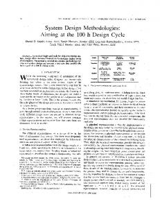
to exist, the corresponding entry in C is given a “score” that attempts to describe the relationship. For example, in the example given by Hauser [9] the relationship could be “strong positive”, “medium positive”, “medium negative”, or “strong negative”. In the case study that is to follow, the system of scoring is completely different. The type of scoring system to be used is left up to the designer to decide. The final part of the House, Section D, is the roof matrix where the user can assess interdependencies among the engineering attributes. Again, the scoring used to describe the relationship is user defined.

D B

A

C

Figure 1. Generic House of Quality The major problem with HoQ is the way in which the attribute relations are established through arbitrary scales. While it may be possible for designers to identify possible relationships in a qualitative sense, i.e., strong or weak and/or positive or negative, there is no reason to believe that the scale chosen actually captures the relationship appropriately on a quantitative level. For example, consider part of the HoQ for the design of a Spirometer, taken from Hauser [29] and shown in Figure 2. The scoring scale used is (1, 3, 9) for (weak, medium, strong) relationships respectively. However, the scale used is not restricted to (1, 3, 9). In fact, any scale could be applied, such as (2, 5, 8) and in the literature, it is often the case that other permutations of three numbers from 1 to 9 are used. In this research it is hypothesized that none of these scales are appropriate since they are arbitrary. The use of arbitrary scales in HoQ is in violation of the second element of validity, in that there is no meaningful information captured by the model. The fact that the scales are arbitrary means that the true relationship between the customer and engineering attributes is unknown. In fact, it has been suggested that the use of such scales is no better than using a random number generator2. Evidence of this is offered in the case study but first a review of Axiomatic Design is provided.

As stated, this definition is a starting point and is certainly subject to debate and change. In this paper however, it represents the definition of validation under which two decision-support methods, House of Quality and Suh’s Axiomatic Design, are evaluated. Before evaluating these methods the basics of each is reviewed and a discussion of how they violate the definition of validity is provided. House of Quality (HoQ) The House of Quality represents the basic design tool of the management philosophy known as Quality Function Deployment (QFD) [9]. HoQ represents a conceptual map whose goal is to find the relationship between the customer attributes and the engineering attributes of a product. The objective is to set targets for the engineering attributes and understand the importance of each engineering attribute based on the relationship between the two domains [9]. The phrase “House of Quality” comes from the basic graphical structure shown in Figure 1. Section A of the House represents the customer attributes, which are listed down the rows of the matrix structure. Section B represents the engineering attributes, which are listed across the columns of the matrix structure. Section C is the relationship matrix, where the effect of each engineering attribute from B on each customer attribute from A is determined. If a relationship between a particular customer and engineering attribute is said

2 This idea originated in the National Science Foundation Open Workshop on Decision Based Design through dialogue with Dr. George Hazelrigg.

3

Copyright © 2003 by ASME

“coupled” or the FRs cannot be satisfied [15]. These three cases are shown in Figure 3. FR1 FR2 FR3

=

1 0 0

0 1 0

0 0 1

DP1 DP2 DP3

Uncoupled

FR1 FR2 FR3

=

1 0 0

1 1 0

1 1 1

DP1 DP2 DP3

Decoupled

FR1 FR2 FR3

=

1 1 1

1 1 0

0 1 1

DP1 DP2 DP3

Coupled

Figure 3. Uncoupled, decoupled, and coupled designs. For any given design matrix, it is possible to find a quantitative measure of the independence. Suh gives two measures of independence, reangularity, R, and semangularity, S. Reangularity “measures the orthogonality between the DPs” and can be thought of as a measure of the interdependence among DPs. Semangularity measures the “angular relationship between the corresponding axes of DPs and FRs” and can be thought of as a measure of the correlation between one FR and any pair of DPs [15]. Both have a maximum value of unity, which corresponds to an uncoupled (ideal) design. As the level of coupling increases, the reangularity and semangularity decrease. The formulations for each are:

Figure 2. HoQ example [29] Suh’s Axiomatic Design In Suh’s Axiomatic Design, the design world is divided into four different domains [30]: • the customer domain which represents customer attributes (CAs), • the functional domain which represents the functional requirements (FRs), • the physical domain which represents the design parameters (DPs), and • the process domain which represent the process variables (PVs). The goal in Axiomatic Design is to satisfy the goals of the customer domain through accomplishment in the subsequent domains, which requires mapping from one space to the next [30]. In the mapping (design) process, Suh imposes two axioms which must be followed in order to create the “best” design. These axioms are [30]: 1.

The Independence Axiom, which states that the independence of functional requirements must be maintained, and

2.

The Information Axiom, which states that the information content should be minimized.

1

n  2 (∑k =1 DM ki DM kj ) 2   R = ∏ 1− n n 2 2   i =1, n −1 (∑k =1 DM ki ) (∑k =1 DM kj )  j =1+i , n 

  | DM jj | S = ∏ 1 j =1   ∑n Akj2 2  k =1 n

(

)

    

(2)

(3)

Upon satisfying the independence axiom, the next step is to minimize the information content as specified by the second axiom. This is an important step in order to choose the final design from those that have satisfied the first axiom. Information, I, in a systems design context is related to the designer’s specifications (captured by DPs) and the capability of the manufacturing system. The quantitative measure that captures this relation is given by:

To understand the implication of the independence axiom, it is easier to think of the mapping in terms of a linear transformation of the form: {FR} = [DM]{DP} (1) where [DM] represents the design matrix, that maps the functional requirements to the design parameters. The ideal design is one in which the number of FRs equals the number of DPs (square design matrix) and the design matrix is identity. This type of design is referred to as an “uncoupled design”. If the resulting design matrix is upper or lower triangular, the design is referred to as “decoupled”. Finally, if there are off diagonal elements in both the upper and lower triangle or if there are fewer DPs than FRs, the design is referred to as

 system range   I = log   common range 

(4)

where the system range is the capability of the manufacturing system in terms of tolerances and the common range is the overlap between the system range and the design range

4

Copyright © 2003 by ASME

From a validation perspective, the issue with Suh’s Axiomatic Design is that it forces the designer to conform to a particular preference structure. That is, Axiomatic Design not only tells you which attributes to consider in design (independence and information), it also determines the importance (weights) of those attributes. This is in direct violation of the third element of a valid design methodology, i.e., do not bias the designer. Analysis of this is given in the next section. Under the definition of validity established in this work, it has been hypothesized that both the House of Quality and Suh’s Axiomatic Design are flawed design methodologies. In the next section, an evaluation to support these claims is offered in the form of an example problem taken from the literature.

probability density

(tolerance associated with DPs) [15]. This is shown conceptually in Figure 4, where the design and system ranges are represented by probability densities. The more the system and design ranges overlap, the less information content necessary, i.e., the common range and system range are equivalent and the information content from Equation 4 approaches zero.

design range

system range

CASE STUDY In order to prove the statements made in the Background section about the flaws in HoQ and Suh’s Axiomatic Design, the methods are applied to a simple example problem in this section. The example problem is the design of a hair dryer and is taken from Masui [31]. The example problem is given as a House of Quality but the number of customer attributes and engineering attributes is reduced for purposes of simplicity. The resulting HoQ used for the example is shown in Figure 5. The information contained with the relationship matrix is taken directly from the reference. Note that the scale (1, 3, 9) is used to determine the relative weight (importance) of each engineering attribute, as recommended by Hauser [29] and others.

design parameter

common range

Figure 4. Concept of information content.

Engineering Attributes Customer Attributes

air flow

air temperature

dries quickly

9

9

quiet

9

operates easily operates safely comfortable to hold

1

reliable

1

balance (torque)

3 9

3

1

9

volume

number of parts

energy consumption

noise, vibration, electromagnetic wave

Weights

9

9

9

9

9

3

1

1

9

9

3

3

1

9

1

3

physical lifetime

1

9

9

1

3

portable energy efficient

weight

3

9

1

9

1

9

9

9

195

201

93

85

90

9

81

111

148

0.19

0.20

0.09

0.08

0.09

0.01

0.08

0.11

0.15

raw score relative weight

Figure 5. Simplified HoQ for hair dryer design.

5

Copyright © 2003 by ASME

In order to calculate the relative weight for each engineering attribute, first the raw score of each is needed. Raw score for a particular engineering attribute is found by summing the product of the ith “weight” times the ith “score” for a particular column. For example, the raw score for air flow is given as (9×9 + 3×9 + 1×0 + 3×1 + 9×0 + 3×1 + 1×0 + 9×9 = 195). Once the raw score for each engineering attribute is know, the relative weight is calculated by dividing the raw score of the jth engineering attribute by the total of all raw scores. Again, as an example the relative weight for air flow is given as (195 / [195 + 201 + 93 + 85 + 90 + 9 + 81 + 111 + 148] = 0.19). With the background of the design problem understood, the remainder of this section is spent supporting the claims made in the Background section, namely: 1. The House of Quality is flawed because it does not use meaningful information. The scales used are no better than random numbers. 2.

wherever a relationship was found to exist in the original HoQ. In the random HoQ, no provision was made to maintain the level of the relationship. That is, an entry in the original HoQ could be replaced by any number on a continuous scale from 1 to 9 without preserving the a < b < c structure. This process was repeated 84 times and the average raw scores and relative weights for the 84 random cases were calculated. The goal is to show that the random results are no better than the strict scale results. The results of the average weights for the random case are also shown in Table 1. The results in Table 1 strongly support the implication that the arbitrary scales used in HoQ are no better than a random number generator for this design problem. Further, comparison of the results to the original HoQ of Figure 5, also shows little difference. To support the results statistically, t-tests were performed between the average relative weights generated by both the arbitrary scales and the random numbers. A t-test is a quantitative way of testing whether the means of two samples come from the same normal distribution under the assumption of the samples having the same or unique variance [32]. Although the random numbers were taken from a uniform distribution, since calculation of raw scores involves the multiplication of two uniform distributions it is known from the “Law of Large Numbers” that the resulting distribution approaches normal [33]. The null-hypothesis here is that the sample means of the average relative weights is from the same distribution but with different variance and the confidence interval is 95%. The calculation of the t Stat under these assumptions is given by:

Suh’s Axiomatic Design is flawed because it biases the designer by imposing a preference structure.

Empirical Investigation of the House of Quality In order to show that the selected scale in HoQ is no better than a random number generator it is necessary to show that random number insertion is comparable to an arbitrary scoring system. To show this, the following steps were taken. •

HoQ simulation. The total combinations of three number scales (from 1 to 9) were found. Examples include (1, 3, 9), (2, 4, 6), (1, 2, 3), etc. and are always in the form a < b < c, where a is the low score, b the medium score, and c the high score. As stated, this is a combinatorial problem and the number of possible combinations is determined by taking any 3 numbers from 9 (r from n), such that the constraint, a < b < c is met. The number of combinations is found from: n 9 9! n!   = =   = = 84  r  r ! ( n − r )!  3  3! ( 9 − 3 )!

•

HoQ simulation. The original HoQ shown in Figure 5 was recreated 84 times with all the possible combinations. Whenever a 1 appeared in the original HoQ, it was replaced by the lowest score in the current scoring system (a), a 3 in the original HoQ was replaced by the medium score in the current scoring system (b), and a 9 in the original HoQ was replaced by the high score in the current scoring system (c). The raw scores and relative weights were then calculated for each of the 84 cases. This simulates how the HoQ works in reality but the scoring system is not restricted to (1, 3, 9).

•

HoQ simulation. The raw scores and relative weights were then averaged over the 84 cases. The results for the average relative weights are shown in the second column of Table 1.

•

Random HoQ. Next, random numbers taken from a uniform distribution from 1 to 9 were inserted

t=

X1 − X 2  σ 12 σ 22    + n2   n1

(5)

where X’s are the sample means, σ2’s are the sample variances, and n’s are the number of observations in the sample. In the case presented here, X1 is the sample mean of 84 arbitrary scales and X2 is the sample of 84 random number insertions. Similarly, σ12 and σ22 are the arbitrary and random sample variances respectively. In both cases, the number of observations is 84. The t-tests show that the null hypothesis is not false for all the engineering attributes except balance and volume, since the calculated t Stat is greater than t Critical (minimum value that the t Stat must have to uphold null hypothesis). The results of the t-tests are shown in Table 2. Certainly the results generated here should raise some concerns about the use of HoQ as a design tool. The fact that random number generation has produced results similar to the arbitrary scales typically used in HoQ implies that these scales do not provide meaningful information on the relationship between customer and engineering attributes. This contradicts the second element of validation in the Background section. On the other hand, these results tend to illustrate the robustness of HoQ with respect to the weighting scale. In other words, HoQ gives similar results regardless of the weighting scale.

6

Copyright © 2003 by ASME

However, this interpretation of the results implies that a random number generator is at least as good as the weighting scales used by the designers using the method. It is doubtful that any designer or company would feel comfortable prescribing this approach. Despite this problem, the structure of HoQ may still be a valuable design tool if the execution is changed. More on this is covered in the Conclusions section but first a similar empirical study is done using Suh’s Axiomatic Design.

Engineering Attributes air flow air temperature balance weight volume number of parts lifetime energy consumption noise, vibration, electromagnetic wave

Figure 6 shows the structure of Equation 1 applied to the hair dryer design problem of Figure 5. Note that the FRs are a subset of the engineering attributes from the original HoQ. Some DPs that may be found to satisfy this relation are, motor type, fan type, wiring, etc. and the relationship between the FRs and hypothetical DPs would be captured by the design matrix. {FRs}

Average Relative Average Relative Weight (scales) Weight (random) 0.17 0.16 0.18 0.17 0.09 0.10 0.08 0.10 0.07 0.07 0.02 0.03 0.11 0.09 0.10 0.17

Average Relative Average Relative Weight t Stat Weight t Critical 3.12 1.99 3.09 1.99 -0.48 1.99 -5.45 1.99 1.38 1.98 -3.28 1.98 3.57 1.98

-5.87

1.99

Design matrix of size 7 x 7

DP1 DP2 DP3 DP4 DP5 DP6 DP7

Figure 6. Suh’s mapping equation for hair dryer design.

0.19

1.99

{DPs}

energy consumption noise, vibration, electromagnetic wave

0.10

2.31

[DM]

=

lifetime

Table 1. Average results of all scoring combinations.

Engineering Attributes air flow air temperature balance weight volume number of parts lifetime energy consumption noise, vibration, electromagnetic wave

=

air flow air temperature balance weight

Table 2. T-test results for average relative weights. Empirical Investigation of Suh’s Axiomatic Design Here the goal is to show that the axioms on which Suh’s methodology is built biases the designer. To accomplish this, arbitrary design possibilities that map the engineering attributes (FRs) of the HoQ in Figure 5 to hypothetical design parameters (DPs) are created to satisfy the relationship of Equation 1. For convenience, it is assumed that the number of FRs and DPs are equal to one another. In reality, this may require adding DPs or decreasing the number of FRs by combining two or more that are similar. In this case, the number of FRs (engineering attributes) was reduced to seven.

1 0 0 0 0 0 0

1 1 0 0 0 0 0

0 1 1 0 0 0 0

0 1 0 1 0 0 0

0 0 0 1 1 0 0

0 0 0 0 0 1 0

0 0 0 1 1 0 1

1 0 0 0 0 0 0

0 1 0 0 0 0 0

1 1 1 0 0 0 0

0 1 0 1 0 0 0

0 0 1 1 1 0 0

0 0 0 1 0 1 0

0 0 0 1 1 1 1

1 0 0 0 0 0 0

0 1 0 0 0 0 0

0 1 1 0 0 0 0

0 0 1 1 0 0 0

0 0 0 1 1 0 0

0 0 0 0 1 1 0

0 0 0 0 0 0 1

1 0 0 0 0 0 0

0 1 0 0 0 0 0

1 0 1 0 0 0 0

1 0 0 1 0 0 0

0 1 0 1 1 0 0

0 1 0 1 0 1 0

0 0 1 0 0 0 1

R = 0.459 S = 0.144 SR = 0.832 CR = 0.203

R = 0.439 S = 0.083 SR = 0.672 CR = 0.503

R = 0.459 S = 0.250 SR = 0.838 CR = 0.710

R = 0.589 S = 0.118 SR = 0.429 CR = 0.020

Figure 7. Possible design matrices. Figure 7 shows a set of hypothetical design matrices that satisfy the mapping of Figure 6. These do not represent actual designs but rather were generated for the purpose of the empirical investigation conducted here. The reangularity (R), semangularity (S), system range (SR), and common range (CR) are also shown for each design matrix. The reangularity and semangularity were calculated using Equations 2 and 3

7

Copyright © 2003 by ASME

respectively. The system range and common range were arbitrarily selected in order to facilitate the evaluation. To perform the analysis, it is assumed that the design matrix with the highest sum of R and S satisfies the independence axiom, where the ideal (uncoupled) design would have a sum of R and S equal to two. If two of the designs have the same independence measure, then the design that satisfies the information axiom (minimum value for Equation 4) is the best design [15]. Clearly, Suh would choose the third design matrix, since it “maintains independence” more than any other choice, i.e., the sum of R and S is highest. To understand the preference structure that is implied by Suh’s axioms, the problem is converted into an optimization problem with two objectives (Suh’s axioms) and these objectives are integrated into a weighted sum “cost” function, where the objective is to minimize the cost. To accomplish this, the sum of R and S is normalized accordingly to: ||R + S|| = (2 – (R + S))/2

•

•

The results of cases one through three are shown in Table 3. The highlighted entries represent Suh’s design choice by way of the axioms. For Case 1, no matter what the weights used in the cost function (Equation 7), the best design is the same as Suh’s design choice. This makes intuitive sense since the third design matrix is better than all others with respect to both axioms. Now however, consider cases two and three, where the independence measures remain the same as in Figure 6 but the information content has changed. For case two, Suh’s winner is the same as that predicted by the cost function only when the values of w1 are from 0.8 to 1. For case three, the value of w1 must be 0.9 or 1.

(6)

This normalization leads to a value of zero for an ideal (uncoupled) design. The cost function can be represented as: J = w1 ||R + S|| + w2 ||I||

(7)

Where w1 and w2 are weights (whose sum is unity) that capture strength of preference for each axiom and ||I|| is the normalized (divide by biggest entry) value of the information content from Equation 4. Of course this is a simplification of Suh’s axioms but the purpose is to understand how the axioms impart a preference structure on the designer. In order to understand how Suh’s axioms affect the designer preferences, five cases are considered. It should be noted here that each of the hypothetical designs are not related across the five cases. While some of the values of independence or information remain constant from design to design, the designs are considered “different” and the purpose is to show how the preference structure changes. Of course in reality, tolerances and the level of design independence have an interdependent affect on the information content in Suh’s approach. For example, tolerances of an uncoupled design can be changed without affecting the rest of the design. However, as the level of coupling increases, changes made to tolerances on DPs will begin to affect more than one FR. Given this reality, it is necessary to consider the designs independent in the five cases investigated here. The purpose of each case is as follows: • •

•

information content from Case 2. Again, find the weights that correspond to Suh’s winner. Case 4: Three new hypothetical design matrices are compared, where two have the same independence measure but the third is best in information content. The weights are found that correspond to Suh’s winner. Case 5: A fourth design matrix that is best in independence measure but worst in information content is added to the Case 4 scenario and the weights that correspond to Suh’s winner are found.

Case 1 Matrix 1 2 3 4

R 0.459 0.439 0.459 0.589

S 0.144 0.083 0.250 0.118

R+S 0.604 0.523 0.709 0.707

SR 0.832 0.672 0.838 0.429

CR 0.203 0.503 0.710 0.020

I 0.613 0.126 0.072 1.340

||R+S|| 0.698 0.739 0.645 0.646

||I|| 0.458 0.094 0.054 1.000

Case 2 Matrix 1 2 3 4

R 0.459 0.439 0.459 0.589

S 0.144 0.083 0.250 0.118

R+S 0.604 0.523 0.709 0.707

SR 0.832 0.672 0.838 0.429

CR 0.203 0.503 0.357 0.020

I 0.613 0.126 0.371 1.340

||R+S|| 0.698 0.739 0.645 0.646

||I|| 0.458 0.094 0.277 1.000

Case 3 Matrix 1 2 3 4

R 0.459 0.439 0.459 0.589

S 0.144 0.083 0.250 0.118

R+S 0.604 0.523 0.709 0.707

SR 0.832 0.672 0.838 0.429

CR 0.203 0.108 0.123 0.020

I 0.613 0.794 0.833 1.340

||R+S|| 0.698 0.739 0.645 0.646

||I|| 0.458 0.593 0.622 1.000

Table 3. Results of normalization for hypothetical DMs. While the results in Table 3 are strictly hypothetical, they serve the purpose of showing that Suh’s axioms force a preference structure on the designer. As further evidence, consider cases four and five. The results are shown in Table 4. For case four, Suh’s winner is represented by the first entry, since, though it is tied with the second entry in independence measure, it is clearly better in information content. However, using the cost function analysis, the values of w1 must range from 0.6 to 1 in order for this design win. Case five adds another possible design that is the best with regards to independence measures but much worse than all other choice in information content. The only time this new design is the winner is when w1 has a value of 1.

Case 1: Find the necessary weights, w1 and w2 that correspond to Suh’s design choice for the original design matrices of Figure 7. Case 2: Keep the same independence measures (R and S) but change the information content for the design matrices so that Suh’s winner is not better in both independence and information content. Again, find the weights that correspond to Suh’s winner. Case 3: Keep the same independence measures (R and S) but change the information content further for the design matrices so that Suh’s winner is even worse in

8

Copyright © 2003 by ASME

Case 4 Matrix R S R+S SR CR I 1 0.612 0.500 1.112 0.832 0.636 0.117 2 0.612 0.500 1.112 0.672 0.503 0.126 3 0.707 0.354 1.061 0.838 0.686 0.087 Case 5 Matrix 1 2 3 4

R 0.612 0.612 0.707 0.707

S 0.500 0.500 0.354 0.500

R+S 1.112 1.112 1.061 1.207

SR 0.832 0.672 0.838 0.429

CR 0.636 0.503 0.686 0.020

I 0.117 0.126 0.087 1.331

flaws in both the House of Quality and Suh’s Axiomatic Design, two popular design methodologies. The work presented in this paper has brought to light some important concepts in design decision making and uncovered some interesting topics for future research. Specifically,

||R+S|| ||I|| 0.444 1.000 0.444 1.078 0.470 0.745

||R+S|| 0.444 0.444 0.470 0.397

• The empirical study for the hair dryer example showed that a random number generator is just as effective as the arbitrary scales used in the House of Quality. Under the elements of validation defined in this paper, this method is flawed since it does not use meaningful information in relating consumer and engineering attributes. However, the HoQ could be improved if an analytical technique, such as design of experiments was implemented into the matrix structure. This is a topic of future research and has been suggested by Aungst [34]. • Another issue of future investigation is a deeper study of the mechanics behind the HoQ. In the example problem presented in this paper, random numbers were placed in the HoQ matrix where relationships were already known to exist. In future work it is planned to insert random numbers regardless of the existence or non-existence of a relationship between the customer and engineering attributes. This would broaden the results and implications to a wider class of HoQ problems. • The empirical study for the hair dryer also showed that Suh’s Axiomatic Design methodology imposes a preference structure on the designer. Although the cases utilized are “hypothetical”, they serve to represent potential design process data that lead to the preference results of Table 5. Not only do Suh’s axioms dictate which attributes are important (independence and information content), they also effectively select the strengths (weights) that must be associated with these attributes as shown in the five hypothetical cases. While the analytical measures of Suh’s methodology may be useful design tools, the way in which the axioms structure the design process biases the designer. Of course, if this bias matches the designer’s true preferences, then there is no issue of bias. • The hypothetical designs used in the Suh example represent mere possibilities. Future work would include investigation across a pool of actual design problems. There is a need to develop and collect such a “pool” of problems for the design research community to use as benchmark studies for the development and comparison of other design decision methodologies/tools. • The empirical results in this paper should not be thought of as analytical proofs. As discussed in the Background section, design methodologies cannot be proved or disproved in a closed form mathematical way. However, elements of human logic and reason should be used in the evaluation and creation of design decision methods. Continued expansion and understanding of the validation topic represents another element of future research.

||I|| 0.088 0.094 0.065 1.000

Table 4. Results of normalization for other hypothetical DMs. A summary of the results from the five cases is provided in Table 5. The results show the weights in the cost function and the corresponding winner for each case. The highlighted boxes are those instances when the design winner from the cost function is the same as Suh’s. Clearly, the results of this analysis show that Suh’s Axiomatic Design is flawed in the sense that it biases the designer. The bias comes in the form of a preference structure. If this implied preference structure reflects the designer’s true preferences, then this issue of “bias” does not exist. However, if this is not the preference structure of the designer, then this method should not be subscribed to. Changes in the information content affect the importance associated with each axiom (objective) that must be satisfied as shown by cases one through three. Further, designs that are marginally better regarding the independence axiom and much worse on the information axiom are still considered the best design under Suh’s methodology but case five shows that this only occurs when independence is the only decision attribute of interest. w1 0 0.1 0.2 0.3 0.4 0.5 0.6 0.7 0.8 0.9 1

w2 1 0.9 0.8 0.7 0.6 0.5 0.4 0.3 0.2 0.1 0

Winning Design via Cost Function Case 1 Case 2 Case 3 Case 4 Case 5 3 2 1 3 3 3 2 1 3 3 3 2 1 3 3 3 2 1 3 3 3 2 1 3 3 3 2 1 1 3 3 2 1 1 1 3 2 1 1 1 3 3 1 1 1 3 3 3 1 1 3 3 3 1&2 4

Table 5. Summary of results for Axiomatic Design evaluation. While simple in nature, the empirical evaluations performed here on HoQ and Suh’s Axiomatic Design show that these approaches to design decision making are flawed under the elements of validity given in the Background section. In the next section, some general conclusions on the research presented in this paper and future research issues are discussed.

The hope is that this paper raises the level of awareness for what should be an important issue in engineering design, namely, the validation of design decision methodologies. The expectation is that this research will further the work started by others and improve the way in which design decisions are made by encouraging the research community to critically evaluate the process under which these decisions are made.

CONCLUSIONS The goal in this paper was to make a case for the validation of decision support methodologies. The justification for validation is given in the case study, which empirically shows

9

Copyright © 2003 by ASME

the 18th Annual Meeting of the American Society for Engineering Management, pp. 73-79. [17] Saari, D.G., 2000, “Mathematical Structure of Voting Paradoxes. I; Pair-wise Vote. II; Positional Voting,” Economic Theory, 15, pp. 1-103. [18] Kimbleton, S., 1972, “The Role of Computer System Models in Performance Evaluation,” Association for Computing Machinery, Inc. [19] Bell, D., Raiffa, H. & Tversky, A., 1988, “Descriptive, normative, and prescriptive interactions in decision making,” In: Decision making: Descriptive, normative, and prescriptive interactions, eds. D. Bell, H. Raiffa & A. Tversky, Cambridge University Press, pp. 9-30. [20] Hazelrigg, G., 1996, Systems Engineering: An Approach to Information-Based Design, Prentice Hall, Upper Saddle River, NJ, pp. 357-358. [21] Baron, S., Kruser, D., and Huey, B., 1990, Quantitative Modeling of Human Performance in Complex, Dynamic Systems, Panel on Human Performance Modeling, Committee on Human Factors, National Research Council. [22] Merriam Webster Online Dictionary, 2003, http://www.m-w.com. [23] Pedersen, K., Emblemsvag, J., Bailey, R., Allen, J., and Mistree, F., 2000, “Validating Design Methods and Research: The Validation Square,” ASME Design Theory and Methodology, Baltimore, MD, DETC2000/DTM-14579. [24] Matheson, D. and Matheson, J., 1998, The Smart Organization: Creating Value Through Strategic R&D, Harvard Business School Press, Boston MA, pp.44. [25] Simpson, T. W., Rosen, D., Allen, J. K., and Mistree, F., 1998, “Metrics for Assessing Design Freedom and Information Certainty in the Early Stages of Design,” Journal of Mechanical Design, 120, No. 4, pp. 628-635. [26] Starr, P. J., 1991, “The Design Process as Managing an Open System of Information,” ASME Design Theory and Methodology Conference, Miami, FL, ASME, DE 31, pp. 285289. [27] Scott, M., and Antonsson, E., 1998, “Aggregation Functions for Engineering Design Tradeoffs,” Fuzzy Sets and Systems, 99, No. 3, pp. 253-264. [28] Altshuller, G., 1999, The Innovation Algorithm: TRIZ, Systematic Innovation and Technical Creativity, Technical Innovation Center, Worchester, MA. [29] Hauser, J., 1993, “How Puritan-Bennet Used the House of Quality,” Sloan Management Review, Spring 1993. [30] Suh, N.P., 1995, “Axiomatic Design of Mechanical Systems,” Journal of Mechanical Design, 117, No 2, pp. S2(9). [31] Masui, K., Sakao, T., Aizawa, S., and Inaba, A., 2002, “Quality Function Deployment for Environment (QFDE) to Support Design for Environment (DFE),” ASME Design for Manufacturing, Montreal, Canada, DETC2002/DFM-34199. [32] Dunn, O., and Clark, V., 1987, Applied Statistics: Analysis of Variance and Regression, Second Edition, John Wiley and Sons, New York. [33] Guttman, I., Wilks, S., and Hunter, J., 1965, Introductory Engineering Statistics, John Wiley and Sons, New York, pp. 105-106. [34] Aungst, S., Barton, R., and Wilson, D.T., 2002, “Integrating Marketing Models,” Institute for the Study of Business Markets, Penn State University, ISBM Report 122002.

ACKNOWLEDGMENTS We gratefully acknowledge the National Science Foundation, grant DMII-9875706, in support of this research. A special acknowledgment also goes to Dr. George Hazelrigg and Dr. Don Saari, as their thoughts and insights revealed at the National Science Foundation Open Workshop for Decision Based Design went a long way in influencing the ideas in this paper. REFERENCES [1] Shupe, J. A., Muster, D., Allen, J. K. and Mistree, F., 1988, “Decision-Based Design: Some Concepts and Research Issues” in Expert Systems, Strategies and Solutions in Manufacturing Design and Planning, pp. 3-37, (A. Kusiak, Ed.), Dearborn, Michigan: Society of Manufacturing Engineers. [2] Hazelrigg, G.A., 1998, “A Framework for DecisionBased Engineering Design,” Journal of Mechanical Design, 120, pp. 653-658. [3] Marston, M. and Mistree, F., 1998, “An Implementation of Expected Utility Theory in Decision Based Design”, ASME Design Theory and Methodology, Atlanta, GA, DETC98/DTM-5670. [4] Gu, X., Renaud, J., Ashe, L., and Batill, S., 2000, “Decision-Based Collaborative Optimization under Uncertainty,” ASME Design Automation Conference, Baltimore, MD, DETC2000/DAC-14297. [5] Roser, C. and Kazmer, D., 2000, “Flexible Design Methodology,” ASME Design for Manufacturing Conference, Baltimore, MD, DETC00/DFM-14016. [6] Olewnik, A. Brauen, T., Ferguson, S., and Lewis, K., 2001, “A Framework for Flexible Systems and its Implementation in Multiattribute Decision Making”, ASME Design Theory And Methodology Conference, Pittsburgh, Pa., DETC2001/DTM-21703. [7] Wassenaar, H. J., and Chen, W., 2001, “An Approach to Decision-Based Design,” ASME Design Theory and Methodology, Pittsburgh, PA, DETC2001/DTM-21683. [8] Terniko, J., 1996, Step by Step QFD: Customer Driven Product Design, Responsible Management, Inc., Nottingham, NH. [9] Hauser, J. and Clausing, D., 1988, “The House of Quality,” Harvard Business Review, 66, Issue 3, pp. 63 (11). [10] Pugh, S., 1996, Creating Innovative Products Using Total Design, Addison-Wesley Publishing Company, Reading, MA. [11] Saaty, T., 1980, The Analytical Hierarchy Process, McGraw-Hill. [12] Keeney, Ralph and Raiffa, Howard, 1993, Decisions With Multiple Objectives: Preferences and Value Tradeoffs, Cambridge University Press, United Kingdom. [13] Messac, A., 1996, “Physical Programming: Effective Optimization for Computational Design,” AIAA Journal, 34, No. 1, pp.149-158. [14] Taguchi, G., 1986, “Introduction to Quality Engineering,” Asian Productivity Organization (Distributed by American Supplier Institute, Inc.), Dearborn, MI. [15] Suh, N., 1990, The Principles of Design, Oxford University Press, New York. [16] Barzalai, J., 1997, “A New Methodology for Dealing with Conflicting Engineering Design Criteria”, Proceedings of

10

Copyright © 2003 by ASME