One-Class LP Classifier for Dissimilarity Representations
1
El˙zbieta P˛ekalska1 , David M.J.Tax2 and Robert P.W. Duin1 Delft University of Technology, Lorentzweg 1, 2628 CJ Delft, The Netherlands 2 Fraunhofer Institute FIRST.IDA, Kekuléstr.7, D-12489 Berlin, Germany
[email protected],
[email protected]
Abstract Problems in which abnormal or novel situations should be detected can be approached by describing the domain of the class of typical examples. These applications come from the areas of machine diagnostics, fault detection, illness identification or, in principle, refer to any problem where little knowledge is available outside the typical class. In this paper we explain why proximities are natural representations for domain descriptors and we propose a simple one-class classifier for dissimilarity representations. By the use of linear programming an efficient one-class description can be found, based on a small number of prototype objects. This classifier can be made (1) more robust by transforming the dissimilarities and (2) cheaper to compute by using a reduced representation set. Finally, a comparison to a comparable one-class classifier by Campbell and Bennett is given.
1 Introduction The problem of describing a class or a domain has recently gained a lot of attention, since it can be identified in many applications. The area of interest covers all the problems, where the specified targets have to be recognized and the anomalies or outlier instances have to be detected. Those might be examples of any type of fault detection, abnormal behavior, rare illnesses, etc. One possible approach to class description problems is to construct oneclass classifiers (OCCs) [13]. Such classifiers are concept descriptors, i.e. they refer to all possible knowledge that one has about the class. An efficient OCC built in a feature space can be found by determining a minimal volume hypersphere around the data [14, 13] or by determining a hyperplane such that it separates the data from the origin as well as possible [11, 12]. By the use of kernels [15] the data is implicitly mapped into a higher-dimensional inner product space and, as a result, an OCC in the original space can yield a nonlinear and non-spherical boundary; see e.g. [15, 11, 12, 14]. Those approaches are convenient for data already represented in a feature space. In some cases, there is, however, a lack of good or suitable features due to the difficulty of defining them, as e.g. in case of strings, graphs or shapes. To avoid the definition of an explicit feature space, we have already proposed to address kernels as general proximity measures [10] and not only as symmetric, (conditionally) positive definite functions of two variables
[2]. Such a proximity should directly arise from an application; see e.g. [8, 7]. Therefore, our reasoning starts not from a feature space, like in case of the other methods [15, 11, 12, 14], but from a given proximity representation. Here, we address general dissimilarities. The basic assumption that an instance belongs to a class is that it is similar to examples within this class. The identification procedure is realized by a proximity function equipped with a threshold, determining whether an instance is a class member or not. This proximity function can be e.g. a distance to an average representative, or a set of selected prototypes. The data represented by proximities is thus more natural for building the concept descriptors, i.e. OCCs, since the proximity function can be directly built on them. In this paper, we propose a simple and efficient OCC for general dissimilarity representations, discussed in Section 2, found by the use of linear programming (LP). Section 3 presents our method together with a dissimilarity transformation to make it more robust against objects with large dissimilarities. Section 4 describes the experiments conducted, and discusses the results. Conclusions are summarized in Section 5.
2 Dissimilarity representations Although a dissimilarity measure D provides a flexible way to represent the data, there are some constraints. Reflectivity and positivity conditions are essential to define a proper measure; see also [10]. For our convenience, we also adopt the symmetry requirement. We do not require that D is a strict metric, since non-metric dissimilarities may naturally be found when shapes or objects in images are compared e.g. in computer vision [4, 7]. Let z and pi refer to objects to be compared. A dissimilarity representation can now be seen as a dissimilarity kernel based on the representation set R = {p 1 , .., pN } and realized by a mapping D(z, R) : F → RN , defined as D(z, R) = [D(z, p1 ) . . . D(z, pN )]T . R controls the dimensionality of a dissimilarity space D(·, R). Note also that F expresses a conceptual space of objects, not necessarily a feature space. Therefore, to emphasize that objects, like z or pi , might not be feature vectors, they will not be printed in bold. The compactness hypothesis (CH) [5] is the basis for object recognition. It states that similar objects are close in their representations. For a dissimilarity measure D, this means that D(r, s) is small if objects r and s are similar.If we demand that D(r, s) = 0, if and only if the objects r and s are identical, this implies that they belong to the same class. This can be extended by assuming that all objects s such that D(r, s) < ε, for a sufficient small ε, are so similar to r that they are members of the same class. Consequently, D(r, t) ≈ D(s, t) for other objects t. Therefore, for dissimilarity representations satisfying the above continuity, the reverse of the CH holds: objects similar in their representations are similar in reality and belong, thereby, to the same class [6, 10]. Objects with large distances are assumed to be dissimilar. When the set R contains objects from the class of interest, then objects z with large D(z, R) are outliers and should be remote from the origin in this dissimilarity space. This characteristic will be used in our OCC. If the dissimilarity measure D is a metric, then all vectors D(z, R), lie in an open prism (unbounded from above1), bounded from below by a hyperplane on which the objects from R are. In principle, z may be placed anywhere in the dissimilarity space D(·, R) only if the triangle inequality is completely violated. This is, however, not possible from the practical point of view, because then both the CH and its reverse will not be fulfilled. Consequently, this would mean that D has lost its discriminating properties of being small for similar objects. Therefore, the measure D, if not a metric, has to be only slightly nonmetric (i.e. the triangle inequalities are only somewhat violated) and, thereby, D(z, R) will still lie either in the prism or in its close neigbourhood. 1
the prism is bounded if D is bounded
3 The linear programming dissimilarity data description To describe a class in a non-negative dissimilarity space, one could minimize the volume of the prism, cut by a hyperplane P : w T D(z, R) = ρ that bounds the data from above2 (note that non-negative dissimilarities impose both ρ ≥ 0 and wi ≥ 0). However, this might be not a feasible task. A natural extension is to minimize the volume of a simplex with the main vertex being the origin and the other vertices v j resulting from the intersection of P and the axes of the dissimilarity space (v j is a vector of all zero elements except for vji = ρ/wi , given that wi 6= 0). Assume now that there are M non-zero weights of the hyperplane P , so effectively, P is constructed in a RM . From geometry we know that the volume V of such a simplex can be expressed as V = (VBase /M !) · (ρ/||w||2 ), where VBase is the volume of the base, defined by the vertices v j . The minimization of h = ρ/||w||2 , i.e. the Euclidean distance from the origin to P , is then related to the minimization of V . Let {D(pi , R)}N i=1 , N = |R| be a dissimilarity representation, bounded by a hyperplane P , i.e. wT D(pi , R) ≤ ρ for i = 1, . . . , N , such that the Lq distance to the origin dq (0, P ) = ρ/||w||p is the smallest (i.e. q satisfies 1/p + 1/q = 1 for p ≥ 1) [9]. This means that P can be determined by minimizing ρ − ||w||p . However, when we require ||w||p = 1 (to avoid any arbitrary scaling of w), the construction of P can be solved by the minimization of ρ only. The mathematical programming formulation of such a problem is [9, 1]: min ρ (1) s.t. wT D(pi , R) ≤ ρ, i = 1, 2, .., N, ||w||p = 1, ρ ≥ 0. If p = 2, then P is found such that h is minimized, yielding a quadratic optimization problem. A much simpler √ LP formulation, realized for p = 1, is of our interest. Knowing that ||w||2 ≤ ||w||1 ≤ M||w||2 and by√the assumption of ||w||1 = 1, after simple calculations, we find that ρ ≤ h = ρ/||w||2 ≤ M ρ. Therefore, by minimizing d∞ (0, P ) = ρ, (and ||w||1 = 1), h will be bounded and the volume of the simplex considered, as well. By the above reasoning and (1), a class represented by dissimilarities can be characterized by a linear proximity function with the weights w and the threshold ρ. Our one-class classifier CLPDD , Linear Programming Dissimilarity-data Description, is then defined as: CLPDD (D(z, ·)) = I(
X
wj D(z, pj ) ≤ ρ),
(2)
wj 6=0
where I is the indicator function. The proximity function is found as the solution to a soft margin formulation (which is a straightforward extension of the hard margin case) with ν ∈ (0, 1] being the upper bound on the outlier fraction for the target class: PN min ρ + ν 1N i=1 ξi (3) s.t. wT D(pi , R) ≤ ρ + ξi , i = 1, 2, .., N P j wj = 1, wj ≥ 0, ρ ≥ 0, ξi ≥ 0. In the LP formulations, sparse solutions are obtained, meaning that only some w j are positive. Objects corresponding to such non-zero weights, will be called support objects (SO).
The left plot of Fig. 1 is a 2D illustration of the LPDD. The data is represented in a metric dissimilarity space, and by the triangle inequality the data can only be inside the prism indicated by the dashed lines. The LPDD boundary is given by the hyperplane, as close to the origin as possible (by minimizing ρ), while still accepting (most) target objects. By the discussion in Section 2, the outliers should be remote from the origin. Proposition. In (3), ν ∈ (0, 1] is the upper bound on the outlier fraction for the target class, i.e. the fraction of objects that lie outside the boundary; see also [11, 12]. This means that 1 PN i=1 (1 − CLPDD (D(pi , ·)) ≤ ν. N 2
P is not expected to be parallel to the prism’s bottom hyperplane
D(. ,p j)
LPDD: minρ
T
LPSD: min 1/N sum k(w K(xk ,S) + ρ )
K(.,x j)
ρ
1
−ρ || w ||1 = 1
w
0
Dissimilarity space
D(.,p i)
w
0
Similarity space
1
K(.,x i)
Figure 1: Illustrations of the LPDD in the dissimilarity space (left) and the LPSD in the similarity space (right). The dashed lines indicate the boundary of the area which contains the genuine objects. The LPDD tries to minimize the max-norm distance from the bounding hyperplane to the origin, while the LPSD tries to attract the hyperplane towards the average of the distribution.
The proof goes analogously to the proofs given in [11, 12]. Intuitively, the proof P follows this: assume we have found a solution of (3). If ρ is increased slightly, the term i ξi in the objective function will change proportionally to the number of points that have non-zero ξ i (i.e. the outlier objects). At the optimum of (3) it has to hold that N ν ≥ #outliers. Scaling dissimilarities. If D is unbounded, then some atypical objects of the target class (i.e. with large dissimilarities) might badly influence the solution of (3). Therefore, we propose a nonlinear, monotonous transformation of the distances to the interval [0, 1] such that locally the distances are scaled linearly and globally, all large distances become close to 1. A function with such properties is the sigmoid function (the hyperbolical tangent can also be used), i.e. Sigm(x) = 2/(1 + e−x/s ) − 1, where s controls the ’slope’ of the function, i.e. the size of the local neighborhoods. Now, the transformation can be applied in an element-wise way to the dissimilarity representation such that Ds (z, pi ) = Sigm(D(z, pi )). Unless stated otherwise, the CLPDD will be trained on Ds . A linear programming OCC on similarities. Recently, Campbell and Bennett have proposed an LP formulation for novelty detection [3]. They start their reasoning from a feature space in the spirit of positive definite kernels K(S, S) based on the set S = {x1 , .., xN }. They restricted themselves to the (modified) RBF kernels, i.e. for 2 2 K(xi , xj ) = e−D(xi ,xj ) /2 s , where D is either Euclidean or L1 (city block) distance. In principle, we will refer to RBFp , as to the ’Gaussian’ kernel based on the Lp distance. Here, to be consistent with our LPDD method, we rewrite their soft-margin LP formulation (a hard margin formulation is then obvious), to include a trade-off parameter ν (which lacks, however, the interpretation as given in the LPDD), as follows: PN PN min N1 i=1 (wT K(xi , S) + ρ) + ν 1N i=1 ξi T (4) s.t. w K(xi , S) + ρ ≥ −ξi , i = 1, 2, .., N P j wj = 1, wj ≥ 0, ξi ≥ 0. Since K can be any similarity representation, for simplicity, we will call this method Linear Programming Similarity-data Description (LPSD). The CLPSD is then defined as: CLPSD (K(z, ·)) = I(
X
wj K(z, xj ) + ρ ≥ 0).
(5)
wj 6=0
In the right plot of Fig. 1, a 2D illustration of the LPSD is shown. Here, the data is represented in a similarity space, such that all objects lie in a hypercube between 0 and 1. Objects remote from the representation objects will be close to the origin. The hyperplane is optimized to have minimal average output for the whole target set. This does not necessarily mean a good separation from the origin or a small volume of the OCC, possibly resulting in an unnecessarily high outlier acceptance rate.
LPDD on the Euclidean representation s = 0.3
1.5
s = 0.4
1.5
s = 0.5
1.5
s=1
1.5
1
1
1
1
0.5
0.5
0.5
0.5
0.5
0
0
0
0
0
−0.5
−0.5
−0.5
−0.5
−0.5
−0.5
0
0.5
1
−0.5
0
0.5
1
−0.5
0
0.5
1
−0.5
0
0.5
s=3
1.5
1
1
−0.5
0
0.5
1
LPSD based on RBF2 s = 0.3
1.5
s = 0.4
1.5
s = 0.5
1.5
s=1
1.5
1
1
1
1
0.5
0.5
0.5
0.5
0.5
0
0
0
0
0
−0.5
−0.5
−0.5
−0.5
−0.5
−0.5
0
0.5
1
−0.5
0
0.5
1
−0.5
0
0.5
1
−0.5
0
0.5
s=3
1.5
1
1
−0.5
0
0.5
1
Figure 2: One-class hard margin LP classifiers for an artificial 2D data. From left to right, s takes the values of 0.3d, 0.4d, 0.5d, d, 3d, where d is the average distance. Support objects are marked by squares.
Extensions. Until now, the LPDD and LPSD were defined for square (dis)similarity matrices. If the computation of (dis)similarities is very costly, one can consider a reduced representation set Rred ⊂ R, consisting of n