One-Loop Calculations with BlackHat - SLAC - Stanford University

July 2008 MIT-CTP 3963 Saclay-IPhT-T08/117 SLAC-PUB-13295 UCLA/08/TEP/21

One-Loop Calculations with BlackHat C. F. Bergera , Z. Bernb , L. J. Dixonc , F. Febres Corderob, D. Fordec , H. Itab , D. A. Kosowerd∗ , D. Maˆıtrec† a

Center for Theoretical Physics, Massachusetts Institute of Technology, Cambridge, MA 02139, USA

b

Department of Physics and Astronomy, UCLA, Los Angeles, CA 90095-1547, USA

c

Stanford Linear Accelerator Center, Stanford University, Stanford, CA 94309, USA

d

Institut de Physique Th´eorique, CEA–Saclay, F–91191 Gif-sur-Yvette cedex, France

We describe BlackHat, an automated C++ program for calculating one-loop amplitudes, and the techniques used in its construction. These include the unitarity method and on-shell recursion. The other ingredients are compact analytic formulae for tree amplitudes for four-dimensional helicity states. The program computes amplitudes numerically, using analytic formulæ only for the tree amplitudes, the starting point for the recursion, and the loop integrals. We make use of recently developed on-shell methods for evaluating coefficients of loop integrals, in particular a discrete Fourier projection as a means of improving numerical stability. We illustrate the good numerical stability of this approach by computing six-, seven- and eight-gluon amplitudes in QCD and comparing against known analytic results.

vector bosons), precision calculations at next-tonext-to-leading order (NNLO) are needed. For other processes, NLO will likely suffice until the LHC enters its precision-measurement era. There are a large number of processes that ought to be computed, however, and these include many processes with many final-state jets, corresponding to large final-state parton multiplicity. NLO predictions can be provided by partonlevel Monte Carlo programs, or by parton showers such as MC@NLO [2]. Both types of program require the computation of virtual and realemission amplitudes. The computation of the latter relies on well-understood technologies [3,4]. Parton-level programs also require the isolation of infrared singularities in the integrated realemission contributions, and a means of canceling them systematically against the virtualcorrection singularities. These technologies [5,6] are also well understood and recently authors have begun to automate them [7]. The infrareddivergent parts of the one-loop virtual corrections are also well-understood [5,8]. The remaining, infrared-finite parts of these one-loop amplitudes have been the difficult part of computations with three final-state objects, and have

1. Introduction Quantitatively reliable predictions for background processes will play an important role in ferreting out signals of new physics in experiments at the upcoming Large Hadron Collider (LHC). New physics beyond the Standard Model is expected to emerge in these TeV-scale experiments. Known-physics backgrounds from electroweak, QCD, and mixed processes will also contribute events that may overwhelm or mimic newphysics signals. Uncovering and understanding the new-physics signals will require use of elaborate kinematic requirements (such as several identified jets, cuts on missing transverse energy, etc.) and reliable knowledge of background processes. Leading-order calculations in QCD suffer from large uncertainties and therefore do not suffice to furnish the required quantitative knowledge of backgrounds. Next-to-leading order calculations are required [1]. Indeed, for a few signal, background, or calibration processes (Higgs-boson production, top production, and distributions associated with production of single electroweak ∗ Presenter † Presenter

Work supported in part by US Department of Energy contract DE-AC02-76SF00515 1

Presented at the 9th Workshop On Elementary Particle Theory: Loops And Legs In Quantum Field Theory 4/20/2008 to 4/25/2008, Sondershausen, Germany Field Theory

2 been the primary bottleneck to computations of processes with four or more final-state objects. BlackHat is one of a new generation of numerical approaches that aims to break this bottleneck. Other numerical efforts along similar lines are described in refs. [9–11]. The traditional approach to one-loop computations uses Feynman diagrams. With an increasing number of external particles, however, the computational complexity of such computations with traditional methods grows factorially. This complexity cannot be tamed by use of technologies such as the spinor-helicity formalism [12] alone. Recent years have witnessed a ferment of development, based on the analytic properties of unitarity and factorization that any amplitude must satisfy, of new approaches to overcoming these computational difficulties [13–18], including onshell methods [19–36]. These methods are efficient, and feature only mild growth in required computer time with increasing number of external particles. They effectively reduce loop calculations to tree-like ones, simplifying them intrinsically and further allowing use of efficient algorithms for the tree-amplitude ingredients.

D. Maˆıtre et al. as distinct from the bespoke analytic process-byprocess calculations that have been done to date. It is also important, however, to obtain an efficient code. As the example of the Berends–Giele recursion relations shows [37], evaluating them recursively with caching of intermediate currents, a numerical approach can make it much more practical to eliminate repeated evaluation of common subexpressions than an analytic approach. Indeed, it seems likely that only a numerical approach can meet the goal of a polynomial-time algorithm for the evaluation of each helicity amplitude at one loop. We begin by separating the amplitude into cutcontaining and rational parts, An = Cn + Rn ,

where the former contain all (poly)logarithms, π 2 terms, and the finite constant in the scalar bubble. The cut-containing part of massless dimensionally-regulated amplitudes with fourdimensional external momenta may be written in a basis of scalar integrals [39–43], X X X Cn = di I4i + ci I3i + bi I2i , (2) i

2. The On-Shell Approach BlackHat is built using an on-shell approach, the unitarity method [19,38] with multiple cuts [20] (a.k.a. generalized unitarity), along with significant refinements [22,30,33] exploiting complex momenta. The cuts replace two or more propagators by delta functions, thus putting the corresponding momenta on shell. They thereby isolate terms in the amplitude with distinct analytic structure, allowing them to be computed independently. We employ a predominantly numerical approach in BlackHat. The loop integrals are evaluated from analytic formulæ, likewise their contributions to residues at spurious singularities (see section 4); and analytic formulæ may be used to speed up evaluation of tree amplitudes. Otherwise, the code is numerical, and in particular everything that corresponds to algebra in a symbolic calculation is done numerically. This makes it easier to design a general-purpose code,

(1)

i

i

The integrals I2,3,4 are respectively bubble, triangle, and box integrals. We compute the coefficients bi , ci , and di numerically using the unitarity method, with fourdimensional loop momenta. The tree amplitudes that feed into the computation may be evaluated efficiently using spinorial methods. We compute the rational parts using loop-level on-shell recursion. 3. Cut Parts The most straightforward coefficients to obtain are those of the box integrals. Imposing four cut conditions on a one-loop integrand, and then setting ǫ = 0, freezes it completely. Furthermore, this isolates the coefficient of a single box integral uniquely. The coefficient is then given [22] in terms of the product of four tree amplitudes at the corners of the box, 1 X σ di = d 2 σ=± i

3

One-loop Calculations with BlackHat dσi

=

tree tree tree tree A(1) A(2) A(3) A(4)

(σ)

li =li

,

(3)

(±)

where the cut loop momenta li are the two solutions to the quadruple-cut on-shell conditions, labeled by σ = ±. In the case of triangle coefficients, we can impose three cut conditions. Here, the cut conditions no longer freeze the integrand completely; one degree of freedom is left over. There are different ways to parametrize this degree of freedom [14,30]; we use the variant proposed by Forde [33], e µ e e µ +K e µ + t hK e 1 |γ µ |K e 3 i+ hK3 |γ |K1 i ,(4) lµ (t) = K 1 3 2 2t

where K1,3 are the two (possibly massive) external momenta separated √ by the cut propagator l; γ = γ± = −K1 · K3 ± ∆; Si = Ki2 , and γK µ+S1 K3µ e µ γK µ+S3 K1µ eµ =α K ˆ 21 , K3 = −α ˆ ′ 23 , (5) 1 γ − S1 S3 γ − S1 S3

α ˆ=

γS3 (S1 − γ) , S1 S3 − γ 2

α ˆ′ =

γS1 (S3 − γ) . S1 S3 − γ 2

(6)

Once the remaining degree of freedom is parametrized by t, the integrand has the following form, tree tree Atree = (1) A(2) A(3) li =li (t)

c−3 c−2 c−1 + 2 + + c 0 + c 1 t + c 2 t2 + c 3 t3 t3 t t X dσi + . (7) ξiσ (t − tσi ) poles

The sum over poles corresponds to the various box contributions sharing the same triple cuts. We follow Ossola, Papadopoulos, and Pittau (OPP) [30] in subtracting these contributions from the integrand, leaving behind seven independent coefficients. Forde’s parametrization isolates the desired coefficient c0 by virtue of its analytic property — it is the constant as t → ∞, or equivalently it can be extracted as the residue of the integrand divided by t, I dt 1 c0 = T3 (t) . (8) 2πi t

We evaluate this contour integral using a discrete Fourier projection, p   X 1 c0 = T3 t0 e2πij/(2p+1) , (9) 2p + 1 j=−p where t0 is an arbitrary complex number. The projection avoids the potentially-unstable matrix inversion that could arise from simply inverting a system of equations to solve for the seven coefficients c−3 , . . . , c3 . (The other coefficients are needed in order to subtract triangle coefficients when computing in their turn the bubble ones, and can also be obtained by a Fourier projection.) The subtraction of the box coefficients makes the discrete Fourier projection exact and also allows for the flexibility in the choice of t0 . It thereby improves the numerical stability of the calculation. The bubble coefficients can be computed following the same approach, subtracting both box and triangle contributions, and using a twodimensional discrete projection. We refer the reader to ref. [44] for more details. 4. Rational Parts On-shell recursion relations for the rational terms may be derived by considering deformations of the amplitude, parametrized by a complex parameter z [24]. These deformations shift two external momenta by ±z · q where q is a complex null four-vector, so as to preserve overall momentum conservation and leave all external momenta on shell. The recursion relation follows from evaluating the contour integral I Rn (z) 1 dz , (10) Rnlarge z = 2πi C z where C is a circle at infinity. If Rnlarge z does not vanish for a given choice of deformation, it can be computed using an auxiliary recursion relation [27]. The rational terms may be computed using Cauchy’s theorem, X Rn (z) Rn (0) = Rnlarge z − Res . (11) z=zα z poles α

The sum over the poles in the last term can be decomposed into two sets, the physical or spurious

4

D. Maˆıtre et al.

10

-2

Ο(ε )

4

-1

Ο(ε ) 0

10

10

Ο(ε )

3

--++++

--+++++

--++++++

2

10

10

1

0

-16 -14 -12 -10 -8

-6

-4

-2

-16 -14 -12 -10 -8

-6

-4

-2

-16 -14 -12 -10 -8

-6

-4

-2

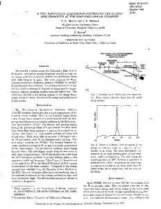
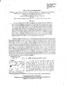
Figure 1. The distribution of the logarithm of the relative error over 100,000 phasespace points for the MHV amplitudes A6 (1− , 2− , 3+ , 4+ , 5+ , 6+ ), A7 (1− , 2− , 3+ , 4+ , 5+ , 6+ , 7+ ) and A8 (1− , 2− , 3+ , 4+ , 5+ , 6+ , 7+ , 8+ ). The dashed (black) curve in each histogram gives the relative error for the 1/ǫ2 part, the solid (red) curve gives the 1/ǫ singularity, and the shaded (blue) distribution gives the finite ǫ0 component of the corresponding helicity amplitude.

poles, depending on whether the pole is or is not present in the full deformed one-loop amplitude, Rn = RnD + RnS + Rnlarge z .

(12)

The contributions RnD from the physical poles can be computed using on-shell recursive diagrams [26]. In BlackHat, the residues at the spurious poles are computed using the cut parts. Because the spurious poles must cancel in the amplitude as a whole, we have X X Rn (z) Cn (z) RnS = − Res = Res , (13) z z z z β β spur. spur. poles β

poles β

where Cn (z) is the cut part from eq. (1), as deformed by the on-shell deformation parametrized by z. The spurious singularities arise from zeros of Gram determinants implicitly appearing in the denominators of the integral coefficients bi , ci , and di of eq. (2). We evaluate the residues of these singularities by making a discrete approximation to a contour integral on a small circle around the

pole. At each complex value on the circle, we evaluate the coefficients bi , ci , and di numerically as described in the previous section. Since the residues are of course rational, and can only arise from expanding the dilogarithms or logarithms in the integral functions, we do not directly evaluate the loop integrals numerically; rather, we first expand them analytically in the appropriate neighborhood of the Gram-determinant singularity, and then evaluate the rational expansion coefficients numerically. We can control the approximation by choosing the size of the circles around the spurious singularity and the number of points on the circle. (The current code evaluates the integrand at ten points around the circle.) This risks numerical instabilities if the circle becomes too small. In order to handle possible numerical instabilities, we test for them dynamically, that is event by event and spurious pole by spurious pole. We test to see that the coefficient of the non-logarithmic 1/ǫ singularity is reproduced correctly. It is sufficient to test the bubble coeffi-

5

One-loop Calculations with BlackHat cients, because they produce this singular term. Box and triangle coefficients are tested indirectly, because they are subtracted in order to compute the bubble coefficients. We also test to see that the spurious singularities cancel in the sum over bubble coefficients. If either of these tests fail, we recompute the numerically unstable terms of the amplitude at higher precision. Because the fraction of points failing the tests is small, this does not impose a significant time penalty on our code. 5. Results As an example, we used BlackHat to compute the one-loop 2 → 4-, 2 → 5-, and 2 → 6gluon maximally helicity-violating (MHV) amplitudes for nf = 0 at 100,000 phase-space points, generated using a flat distribution. √ (We impose the following cuts: ET > 0.01 s, η < 3, and ∆R > 0.4.) We compared the numerical results against those computed using known analytic results. The histogram in fig. 1 shows the results. The horizontal axis gives the logarithmic relative error,  num  |An − Atarget | n , (14) log10 |Atarget | n for each of the 1/ǫ2 , 1/ǫ, and ǫ0 parts of the oneloop amplitude. The vertical axis in these plots shows the number of phase-space points in a bin that agree with the target to a specified relative precision. The vertical scale is logarithmic, which enhances the visibility of the tail of the distribution, and thereby illustrates the good numerical stability of the computation. 6. Acknowledgments We thank Academic Technology Services at UCLA for computer support. This research was supported by the US Department of Energy under contracts DE–FG03–91ER40662 and DE– AC02–76SF00515. CFB’s research was supported in part by funds provided by the U.S. Department of Energy (D.O.E.) under cooperative research agreement DE–FC02–94ER40818. DAK’s research is supported by the Agence Nationale

de la Recherce of France under grant ANR–05– BLAN–0073–01. The work of DM was supported by the Swiss National Science Foundation (SNF) under contract PBZH2–117028. REFERENCES 1. Z. Bern et al., 0803.0494 [hep-ph]. 2. S. Frixione and B. R. Webber, JHEP 0206, 029 (2002) [hep-ph/0204244]; S. Frixione, P. Nason and B. R. Webber, JHEP 0308, 007 (2003) [hep-ph/0305252]. 3. F. A. Berends and W. T. Giele, Nucl. Phys. B 306, 759 (1988); F. Caravaglios, M. L. Mangano, M. Moretti and R. Pittau, Nucl. Phys. B 539, 215 (1999) [hepph/9807570]. 4. T. Stelzer and W. F. Long, Comput. Phys. Commun. 81, 357 (1994) [hep-ph/9401258]; A. Kanaki and C. G. Papadopoulos, Comput. Phys. Commun. 132, 306 (2000) [hepph/0002082]; hep-ph/0012004; F. Krauss, R. Kuhn and G. Soff, JHEP 0202, 044 (2002) [hep-ph/0109036]; M. L. Mangano, M. Moretti, F. Piccinini, R. Pittau and A. D. Polosa, JHEP 0307, 001 (2003) [hepph/0206293]; J. Alwall, P. Demin, S. de Visscher, R. Frederix, M. Herquet, F. Maltoni, T. Plehn, D. L. Rainwater, and T. Stelzer, JHEP 0709, 028 (2007) [0706.2334 [hep-ph]]. 5. W. T. Giele and E. W. N. Glover, Phys. Rev. D 46, 1980 (1992); W. T. Giele, E. W. N. Glover and D. A. Kosower, Nucl. Phys. B 403, 633 (1993) [hep-ph/9302225]; S. Frixione, Z. Kunszt and A. Signer, Nucl. Phys. B 467, 399 (1996) [hep-ph/9512328]. 6. S. Catani and M. H. Seymour, Phys. Lett. B 378, 287 (1996) [hep-ph/9602277]; Nucl. Phys. B 485, 291 (1997) [Erratum-ibid. B 510, 503 (1998)] [hep-ph/9605323]. 7. T. Gleisberg and F. Krauss, Eur. Phys. J. C 53, 501 (2008) [0709.2881 [hep-ph]]; M. H. Seymour and C. Tevlin, 0803.2231 [hepph]. 8. Z. Kunszt, A. Signer and Z. Tr´ocs´anyi, Nucl. Phys. B 420, 550 (1994) [hep-ph/9401294]; S. Catani, Phys. Lett. B427:161 (1998) [hepph/9802439].

6 9. G. Ossola, C. G. Papadopoulos and R. Pittau, JHEP 0803, 042 (2008) [0711.3596 [hep-ph]]. 10. R. K. Ellis, W. T. Giele and Z. Kunszt, JHEP 0803, 003 (2008) [0708.2398 [hep-ph]]. 11. W. T. Giele, Z. Kunszt and K. Melnikov, JHEP 0804, 049 (2008) [0801.2237 [hepph]]; R. K. Ellis, W. T. Giele and Z. Kunszt, 0802.4227 [hep-ph]; W. T. Giele and G. Zanderighi, 0805.2152 [hep-ph]; R. K. Ellis, W. T. Giele, Z. Kunszt and K. Melnikov, 0806.3467 [hep-ph]. 12. F. A. Berends, R. Kleiss, P. De Causmaecker, R. Gastmans and T. T. Wu, Phys. Lett. B 103, 124 (1981); P. De Causmaecker, R. Gastmans, W. Troost and T. T. Wu, Nucl. Phys. B 206, 53 (1982); Z. Xu, D. H. Zhang and L. Chang, TUTP-84/3TSINGHUA; R. Kleiss and W. J. Stirling, Nucl. Phys. B 262, 235 (1985); J. F. Gunion and Z. Kunszt, Phys. Lett. B 161, 333 (1985); Z. Xu, D. H. Zhang and L. Chang, Nucl. Phys. B 291, 392 (1987). 13. A. Denner and S. Dittmaier, Nucl. Phys. B 658, 175 (2003) [hep-ph/0212259]; Z. Nagy and D. E. Soper, JHEP 0309, 055 (2003) [hep-ph/0308127]; Phys. Rev. D 74, 093006 (2006) [hep-ph/0610028]; W. T. Giele and E. W. N. Glover, JHEP 0404, 029 (2004) [hep-ph/0402152]; R. K. Ellis, W. T. Giele and G. Zanderighi, Phys. Rev. D 72, 054018 (2005) [Erratum-ibid. D 74, 079902 (2006)] [hep-ph/0506196]; Phys. Rev. D 73, 014027 (2006) [hep-ph/0508308]; C. Anastasiou and A. Daleo, JHEP 0610, 031 (2006) [hepph/0511176]; A. Brandhuber, B. Spence and G. Travaglini, JHEP 0702, 088 (2007) [hepth/0612007]; A. Lazopoulos, K. Melnikov and F. Petriello, Phys. Rev. D 76, 014001 (2007) [hep-ph/0703273]; A. Brandhuber, B. Spence, G. Travaglini and K. Zoubos, JHEP 0707, 002 (2007) [0704.0245 [hep-th]]; M. Moretti, F. Piccinini and A. D. Polosa, 0802.4171 [hepph]. 14. F. del Aguila and R. Pittau, JHEP 0407, 017 (2004) [hep-ph/0404120]. 15. T. Binoth, J. P. Guillet, G. Heinrich, E. Pilon and C. Schubert, JHEP 0510, 015 (2005) [hep-ph/0504267].

D. Maˆıtre et al. 16. A. Denner and S. Dittmaier, Nucl. Phys. B 734, 62 (2006) [hep-ph/0509141]. 17. R. K. Ellis, W. T. Giele and G. Zanderighi, JHEP 0605, 027 (2006) [hep-ph/0602185]. 18. Z. Xiao, G. Yang and C. J. Zhu, Nucl. Phys. B 758, 1 (2006) [hep-ph/0607015]; Nucl. Phys. B 758, 53 (2006) [hep-ph/0607017]; T. Binoth, J. P. Guillet and G. Heinrich, JHEP 0702, 013 (2007) [hep-ph/0609054]. 19. Z. Bern, L. J. Dixon, D. C. Dunbar and D. A. Kosower, Nucl. Phys. B 425, 217 (1994) [hep-ph/9403226]. 20. Z. Bern, L. J. Dixon and D. A. Kosower, Nucl. Phys. B 513, 3 (1998) [hep-ph/9708239]. 21. Z. Bern and A. G. Morgan, Nucl. Phys. B 467, 479 (1996) [hep-ph/9511336]; Z. Bern, L. J. Dixon and D. A. Kosower, Ann. Rev. Nucl. Part. Sci. 46, 109 (1996) [hepph/9602280]; Z. Bern, L. J. Dixon, D. C. Dunbar and D. A. Kosower, Phys. Lett. B 394, 105 (1997) [hep-th/9611127]; Z. Bern, L. J. Dixon and D. A. Kosower, JHEP 0001, 027 (2000) [hep-ph/0001001]. 22. R. Britto, F. Cachazo and B. Feng, Nucl. Phys. B 725, 275 (2005) [hep-th/0412103]. 23. R. Britto, F. Cachazo and B. Feng, Nucl. Phys. B 715, 499 (2005) [hep-th/0412308]. 24. R. Britto, F. Cachazo, B. Feng and E. Witten, Phys. Rev. Lett. 94, 181602 (2005) [hepth/0501052]. 25. Z. Bern, L. J. Dixon and D. A. Kosower, Phys. Rev. D 71, 105013 (2005) [hepth/0501240]; Phys. Rev. D 72, 125003 (2005) [hep-ph/0505055]. 26. Z. Bern, L. J. Dixon and D. A. Kosower, Phys. Rev. D 73, 065013 (2006) [hepph/0507005]. 27. C. F. Berger, Z. Bern, L. J. Dixon, D. Forde and D. A. Kosower, Phys. Rev. D 74, 036009 (2006) [hep-ph/0604195]. 28. C. F. Berger, V. Del Duca and L. J. Dixon, Phys. Rev. D 74, 094021 (2006) [Erratumibid. D 76, 099901 (2007)] [hep-ph/0608180]; S. D. Badger, E. W. N. Glover and K. Risager, JHEP 0707, 066 (2007) [0704.3914 [hep-ph]]. 29. A. Brandhuber, S. McNamara, B. J. Spence and G. Travaglini, JHEP 0510, 011 (2005) [hep-th/0506068]; C. Anastasiou, R. Britto,

One-loop Calculations with BlackHat

30.

31.

32.

33. 34. 35.

36.

37.

38.

39.

40.

B. Feng, Z. Kunszt and P. Mastrolia, Phys. Lett. B 645, 213 (2007) [hep-ph/0609191]; JHEP 0703, 111 (2007) [hep-ph/0612277]. G. Ossola, C. G. Papadopoulos and R. Pittau, Nucl. Phys. B 763, 147 (2007) [hepph/0609007]. R. Britto and B. Feng, Phys. Rev. D 75, 105006 (2007) [hep-ph/0612089]; JHEP 0802, 095 (2008) [0711.4284 [hep-ph]]; R. Britto, B. Feng and P. Mastrolia, 0803.1989 [hep-ph]; R. Britto, B. Feng and G. Yang, 0803.3147 [hep-ph]. Z. Bern, L. J. Dixon and D. A. Kosower, Annals Phys. 322, 1587 (2007) [0704.2798 [hepph]]. D. Forde, Phys. Rev. D 75, 125019 (2007) [0704.1835 [hep-ph]]. G. Ossola, C. G. Papadopoulos and R. Pittau, 0802.1876 [hep-ph]. P. Mastrolia, G. Ossola, C. G. Papadopoulos and R. Pittau, JHEP 0806, 030 (2008) [0803.3964 [hep-ph]]. T. Binoth, G. Ossola, C. G. Papadopoulos and R. Pittau, JHEP 0806 (2008) 082 [0804.0350 [hep-ph]]. R. Kleiss and H. Kuijf, Nucl. Phys. B 312, 616 (1989); D. Forde and D. A. Kosower, Phys. Rev. D 73, 065007 (2006) [hepth/0507292]. Z. Bern, L. J. Dixon, D. C. Dunbar and D. A. Kosower, Nucl. Phys. B 435, 59 (1995) [hep-ph/9409265]. G. ’t Hooft and M. J. G. Veltman, Nucl. Phys. B 153, 365 (1979); G. J. van Oldenborgh and J. A. M. Vermaseren, Z. Phys. C 46, 425 (1990); W. Beenakker and A. Denner, Nucl. Phys. B 338, 349 (1990); A. Denner, U. Nierste and R. Scharf, Nucl. Phys. B 367, 637 (1991); R. K. Ellis and G. Zanderighi, JHEP 0802, 002 (2008) [0712.1851 [hep-ph]]. L. M. Brown and R. P. Feynman, Phys. Rev. 85 (1952) 231; L. M. Brown, Nuovo Cim. 21, 3878 (1961); B. Petersson, J. Math. Phys. 6:1955 (1965); G. K¨ all´en and J. S. Toll, J. Math. Phys. 6:299 (1965); D. B. Melrose, Nuovo Cim. 40, 181 (1965); G. Passarino and M. J. G. Veltman, Nucl. Phys. B 160, 151 (1979); W. L. van Neerven and J. A. M. Ver-

7 maseren, Phys. Lett. B 137, 241 (1984). 41. Z. Bern, L. J. Dixon and D. A. Kosower, Phys. Lett. B 302, 299 (1993) [Erratum-ibid. B 318, 649 (1993)] [hep-ph/9212308]. 42. J. Fleischer, F. Jegerlehner and O. V. Tarasov, Nucl. Phys. B 566, 423 (2000) [hep-ph/9907327]; T. Binoth, J. P. Guillet and G. Heinrich, Nucl. Phys. B 572, 361 (2000) [hep-ph/9911342]. 43. G. Duplan˘ci´c and B. Ni˘zi´c, Eur. Phys. J. C 35, 105 (2004) [hep-ph/0303184]. 44. C. F. Berger, Z. Bern, L. J. Dixon, F. Febres Cordero, D. Forde, H. Ita, D. A. Kosower, D. Maˆıtre 0803.4180 [hep-ph].