Sep 30, 2013 - University of Florida, Gainesville, FL, USA. Email: {walters8 ... approximated using parametric function approximation tech- niques, and an ...
Online Approximate Optimal Path-Following for a Kinematic Unicycle
arXiv:1310.0064v1 [cs.SY] 30 Sep 2013
Patrick Walters, Rushikesh Kamalapurkar, Lindsey Andrews, and Warren E. Dixon
Abstract—Online approximation of an infinite horizon optimal path-following strategy for a kinematic unicycle is considered. The solution to the optimal control problem is approximated using an approximate dynamic programming technique that uses concurrent-learning-based adaptive update laws to estimate the unknown value function. The developed controller overcomes challenges with the approximation of the infinite horizon value function using an auxiliary function that describes the motion of a virtual target on the desired path. The developed controller guarantees uniformly ultimately bounded (UUB) convergence of the vehicle to a desired path while maintaining a desired speed profile and UUB convergence of the approximate policy to the optimal policy. Simulation results are included to demonstrate the controller’s performance.
I. I NTRODUCTION The goal of a mobile robot feedback controller can be classified into three categories: point regulation, trajectory tracking, or path following. Point regulation refers to the stabilization of a dynamical system about a desired state. Trajectory tracking requires a dynamical system to track a time parametrized reference trajectory. Path-following involves convergence of the system state to a given path at a desired speed profile without temporal constraints. Path-following heuristically yields smoother convergence to the desired path and reduces the risk of control saturation [1]. A path-following control structure can also alleviate difficulties in the control of nonholonomic vehicles [2]. Path-following control is particularly useful for mobile robots with objectives that emphasize path convergence and maintaining a desired speed profile (cf. [3]–[9]). To improve path-following performance, optimal control techniques have been applied to path-following. The result in [10] combines line-of-sight guidance and model predictive control (MPC) to optimally follow straight line segments. In [11], the MPC structure is used to develop a controller for an omnidirectional robot with dynamics linearized about the desired path. Nonlinear MPC is used in [12] to develop an optimal path-following controller for a general mobile robot model over a finite time-horizon. In [13], the path-following of a motorcycle is considered using a linear optimal preview control scheme. Patrick Walters, Rushikesh Kamalapurkar, Lindsey Andrews and Warren E. Dixon are with the Department of Mechanical and Aerospace Engineering, University of Florida, Gainesville, FL, USA. Email: {walters8, rkamalapurkar, landr010, wdixon}@ufl.edu This research is supported in part by NSF award numbers 0901491, 1161260, 1217908, ONR grant number N00014-13-1-0151, and a contract with the AFRL Mathematical Modeling and Optimization Institute. Any opinions, findings and conclusions or recommendations expressed in this material are those of the authors and do not necessarily reflect the views of the sponsoring agency.
Approximate dynamic programming-based (ADP-based) techniques have been used to approximate optimal control policies for regulation (cf. [14]–[16]) and trajectory tracking (cf. [17]–[19]). ADP stems from the concept of reinforcement learning and Bellman’s principle of optimality where the solution to the Hamilton-Jacobi-Bellman (HJB) equation is approximated using parametric function approximation techniques, and an actor-critic structure is used to estimate the unknown parameters. Various methods have been proposed in [14]–[23] to approximate the solution to the HJB equation. For an infinite horizon regulation problem, function approximation techniques, such as neural networks (NNs), are used to approximate the value function and the optimal policy. Motivated by the desire to develop a nonlinear optimal path-following control scheme, an ADP-based path-following controller is considered for a kinematic unicycle. The pathfollowing technique in this paper generates a virtual target that is then tracked by the vehicle. The progression of the virtual target along the given path is described by a predefined statedependent ordinary differential equation motivated by [1]. The definition of the virtual target progression in [1] is desired because it relieves a limitation on the initial condition of the vehicle seen in [4], [24], [25]. For an infinite horizon control problem, the state associated with the virtual target progression is unbounded, which presents several challenges. According to the universal function approximation theorem, a NN is a universal approximator for continuous functions on a compact domain. Since the value function and optimal policy depend on the unbounded path parameter, the domain of the approximation is not compact; hence, to approximate the value function using a NN, an alternate description of the virtual target progression that results in a compact domain for the associated state needs to be developed. In addition, the vehicle requires constant control effort to remain on the path; therefore, any control policy that results in path-following also results in infinite cost, rendering the associated control problem ill-defined. In this result, the progression of the virtual target is redefined to remain on a compact domain, and the kinematics of the unicycle are expressed as an autonomous dynamical system in terms of the error between the vehicle and virtual target. A modified control input is developed as the difference between the designed control and the nominal control required to keep the vehicle on the path. The cost function is formulated in terms of the modified control and is defined to exclude the position of the virtual target, so that the vehicle is not penalized for progress along the path. The resulting optimal control
The velocity vector in (2) can be expressed in {f } as �b � d f ~vbf/n = ~vff/n + dt ~ bf/n × ~rbf/f . ~rb/f + ω
𝒚𝒃 unicycle 𝒙𝒃
𝜃𝑏
𝑟𝑏
𝑟𝑏
𝑛
𝑓
𝒔𝒇
𝒚𝒇
𝒚𝒏
The relative position of the� vehicle with �T respect to the virtual where s ∈ R is the target is given as ~rbf/f = s y 0 component along the path’s tangent unit vector sf and y ∈ R is the component along the path’s normal unit vector yf taken at the virtual target’s location. From Figure 1, the velocity of the vehicle expressed in {f } is given as v ~vbf/n = Rθ 0 , (4) 0
path
{𝑏}
𝜃𝑓
{𝑛}
𝒙𝒏
𝑟𝑓
Figure 1.
{𝑓} 𝑛
(3)
where the rotation matrix Rθ : R → R3×3 is defined as cos θ − sin θ 0 Rθ , sin θ cos θ 0 , 0 0 1
virtual target
Description of reference frames.
problem admits admissible solutions, and an autonomous value function that can be approximated on a compact domain, facilitating the development of an online approximation to the optimal controller using the ADP framework. A Lyapunovbased stability analysis is presented to establish uniformly ultimately bounded (UUB) convergence of the vehicle to the path while maintaining the desired speed profile and UUB convergence of the approximate policy to the optimal policy. Simulation results compare the policy obtained using the developed technique to an offline numerical optimal solution for an assessment of performance.
where the angle between {f } and {b} is θ , θb − θf where θf ∈ R is the angle between sf and xn . Substituting (4) into (3) yields 0 s s˙ s˙ p v × y , 0 Rθ 0 = 0 + y˙ + 0 0 0 κ (sp ) s˙ p 0 (5) where sp ∈ R is the arc length the virtual target has moved along the path, and κ : R → R is the path curvature. Based on (5)
II. V EHICLE M ODEL
v cos θ
= s˙ + (1 − κy) s˙ p ,
v sin θ
= y˙ + κss˙ p .
Consider the nonholonomic kinematics for a unicycle given by
(6)
The time derivative of the angle θ is x˙ =
v cos θb ,
y˙ ˙θb
=
v sin θb ,
=
w,
(1)
where x, y ∈ R represent the vehicle’s position in a plane, and θb ∈ R represents the angle between the vehicle’s velocity vector and the x-axis of the inertial frame {n}. The vehicle control inputs are the linear velocity v ∈ R and the angular velocity w ∈ R. A time-varying body reference frame {b} is defined as attached to the vehicle with the x-axis aligned with the vehicle’s velocity vector, as illustrated in Figure 1. Unlike the traditional tracking problem, the path-following objective is to move along a desired path at a specified speed profile. As typical for this class of problems, it is convenient to express the vehicle’s kinematics in a time-varying SerretFrenet reference frame {f } where the origin is fixed to a virtual target on the desired path (cf. [1], [26]). Consider the following vector equation from Figure 1, ~rb/n = ~rf/n + ~rb/f . n d b d The time derivative of ~rb/f is dt ~rb/f = dt ~rb/f + ω ~ b/n × ~rb/f such that �b � d (2) ~vb/n = ~vf/n + dt ~rb/f + ω ~ b/n × ~rb/f .
n d dt θ
=
n d dt θb
n
−
n d dt θf ,
(7)
n
d d where dt θb = w from (1) and dt θf = κs˙ p . Rearranging (6) and augmenting (7) results in the vehicle’s kinematics expressed in {f } given by [1]
s˙ = −s˙ p (1 − κy) + v cos θ, y˙ θ˙
(8)
= −κs˙ p s + v sin θ, = w − κs˙ p .
The location of the virtual target can be determined by projecting the location of the vehicle onto the path. Assuming the projection is well defined, s = 0 and s˙ = 0, and hence from (8) v cos θ s˙ p = . 1 − κy When y = 1/κ, the virtual target’s velocity s˙ p is undefined. Therefore the vehicle’s initial condition is limited to a tube defined by 1/κ along the path, which can be restrictive for paths with large curvature values. Motivated by the development in
[1], instead of projecting the location of the vehicle onto the path, the location of the virtual target is determined by s˙ p , vdes cos θ + k1 s,
(9)
where vdes ∈ R is a desired positive, bounded and timeinvariant speed profile, and k1 ∈ R is an adjustable positive gain. This definition of the virtual target’s speed eliminates the singularity at y = 1/κ. To facilitate the subsequent control development, we define an auxiliary function φ : R → (−1, 1) as φ , tanh (k2 sp ) ,
(10)
where k2 ∈ R is a positive gain. From (9) and (10), the time derivative of φ is � dφ dsp = k2 sech2 tanh−1 (φ) (vdes cos θ + k1 s) . (11) dsp dt Note that the path curvature and desired speed profile can be written as a function of φ. Based on (8) and (11), auxiliary control inputs ve , we ∈ R are designed as ve
, v − vss ,
we
, w − wss ,
(12)
where wss , κvdes and vss , vdes based on the control input required to remain on the path. Substituting (9) and (12) into (8), and augmenting the system state with (11), the closed-loop system expressed in {f } is s˙ = κyvdes cos θ + k1 κsy − k1 s + ve cos θ y˙ θ˙ φ˙
(13)
2
= vdes sin θ − κsvdes cos θ − k1 κs + ve sin θ = κvdes − κ (vdes cos θ + k1 s) + we � = k2 sech2 tanh−1 (φ) (vdes cos θ + k1 s) .
The closed-loop system in (13) can be rewritten in the following control affine form ζ˙ = f (ζ) + g (ζ) u, (14) � �T s y θ φ where ζ = ∈ R4 is the state vector, � �T u = ve we ∈ R2 is the control vector, and the locally Lipschitz functions f : R4 → R4 and g : R4 → R4×2 are defined as κyvdes cos θ + k1 κsy − k1 s vdes sin θ − κsvdes cos θ − k1 κs2 , f (ζ) , κvdes − κ (vdes�cos θ + k1 s) 2 −1 k2 sech tanh (φ) (vdes cos θ + k1 s) cos (θ) 0 sin (θ) 0 . g (ζ) , 0 1 0 0 To facilitate the subsequent stability analysis, define a subset � �T of the state as e = s y θ ∈ R3 .
III. F ORMULATION OF OPTIMAL CONTROL PROBLEM The cost functional for the optimal control problem is defined as ˆ∞ (15) J (ζ, u) = r (ζ (τ ) , u (τ )) dτ, t 4
where r : R → [0, ∞) is the local cost defined as r (ζ, u) = ζ T Qζ + uT Ru. In (15), R ∈ R2×2 is a symmetric positive definite matrix, ¯ ∈ R4×4 is defined as and Q � � Q 03×1 ¯ Q, , 01×3 0 where Q ∈ R3×3 is a positive definite matrix where 2 2 q kξq k ≤ ξqT Qξq ≤ q kξq k , ∀ξq ∈ R3 where q and q are positive constants. The infinite-time scalar value functional V : [0, ∞) → [0, ∞) is written as ˆ∞ V = min
r (ζ (τ ) , u (τ )) dτ,
u∈U
(16)
t
where U is the set of admissible control policies. The objective of the optimal control problem is to determine the optimal policy u∗ that minimizes the cost functional (15) subject to the constraints in (14). Assuming a minimizing policy exists and the value function is continuously differentiable, the Hamiltonian is defined as ∂V (f + gu∗ ) . (17) H , r (ζ, u∗ ) + ∂ζ The Hamilton-Jacobi-Bellman (HJB) equation is given as [27] 0=
∂V + H, ∂t
(18)
where ∂V ∂t ≡ 0 since there exists no explicit dependence on time. The optimal policy is derived from (18) as � �T 1 −1 T ∂V ∗ u =− R g . (19) 2 ∂ζ The analytical expression for the optimal controller in (19) requires knowledge of the value function which is the solution to the HJB. Given the kinematics in (13) and (14), it is unclear how to determine an analytical solution to (18), as is generally the case since (18) is a nonlinear partial differential equation; hence, the subsequent development focuses on the development of an approximate solution. IV. A PPROXIMATE S OLUTION The subsequent development is based on a neural network (NN) approximation of the value function and optimal policy, and follows a similar structure to [16]. The development is included here for completeness. To facilitate the use of a neural network, a temporary assumption is made that the system state lies on a compact set where ζ (t) ∈ χ ⊂ R4 , ∀t ∈ [0, ∞). This
assumption is relieved in the subsequent stability analysis in Remark 1, and is common in NN literature (cf. [28], [29]). Assumption 1. The value function V : R4 → [0, ∞) can be represented by a single-layer NN with L neurons as V (ζ) = W T σ (ζ) + � (ζ) ,
(20)
L
where W ∈ R is the ideal weight vector bounded above by a known positive constant, σ : R4 → RL is a bounded, continuously differentiable activation function, and � : R4 → R is the bounded, continuously differentiable function reconstruction error. From (19) and (20), the optimal policy can be represented as
� 1 (21) u = − R−1 g T σ 0T W + �0T . 2 Based on (20) and (21), the value function and optimal policy NN approximations are defined as ∗
ˆ T σ, Vˆ = W c 1 −1 T 0T ˆ u ˆ = − R g σ Wa , 2
(22) (23)
ˆ c, W ˆ a ∈ RL are estimates of the ideal weight vector where W ˜ c , W −Wc W . The weight estimation errors are defined as W ˜ and Wa , W − Wa . The NN approximation of the Hamiltonian is given as ∂ Vˆ ˆ = r (ζ, u H ˆ) + (f + gˆ u) (24) ∂ζ by substituting (22) and (23) into (17). The Bellman error δ ∈ R is defined as the error between the optimal and approximate Hamiltonian and is given as ˆ − H, δ,H
(25)
where H ≡ 0. Therefore, the Bellman error can be written in a measurable form as T
ˆc ω, δ = r (ζ, u ˆ) + W where ω , σ 0 (f + gˆ u) ∈ RL . Assumption 2. There exists a set of sampled data points {ζj ∈ χ|j = 1, 2, . . . , N } such that ∀t ∈ [0, ∞), N X ωj ωjT = L, rank (26) pj j=1 q where pj , 1 + ωjT ωj denotes the normalization constant, and ωj is evaluated at the specified data point ζj . In general, the rank condition in (26) cannot be guaranteed to hold a priori. However, heuristically, the condition can be met by sampling redundant data, i.e., N � L. Based on PN ωj ωjT Assumption 2, it can be shown that > 0 such j=1 pj that n X ωj ωjT 2 T ξc ≤ c kξc k2 , ∀ξc ∈ R4 c kξc k ≤ ξc p j j=1
even in the absence of persistent excitation [30], [31]. ˆ c in (22) is given by The adaptive update law for W N X ∂δj δj ˆ˙ c = −ηc1 ∂δ δ − ηc2 , W ˆ ˆ p p N ∂ Wc j=1 ∂ Wc j
(27)
where ηc1 , ηc2 ∈ R are positive adaptation gains, ∂∂δ ˆ c = ω is W √ T the regressor matrix, and p , 1 + ω ω is a normalization ˆ a in (23) is given constant. The policy NN update law for W by n � �o ˆ˙ a = proj −ηa W ˆa − W ˆc , W (28) where ηa ∈ R is a positive gain, and proj {·} is a smooth projection operator [32]. Using Assumption 1 and the properties of the projection operator, the policy NN weight estimation errors are bounded above by positive constants. V. S TABILITY A NALYSIS To facilitate the subsequent stability analysis, an unmeasurable from of the Bellman error can be written using (17), (24), and (25), as ˜ cT ω − �0 f + 1 �0 Gσ 0T W + 1 W ˜ aT Gσ W ˜ a + 1 �0 G�0T , δ = −W 2 4 4 (29) where G , gR−1 g T ∈ R4×4 and Gσ , σ 0 Gσ 0T ∈ RL×L are symmetric, positive semi-definite matrices. Similarly, at the sampled points the Bellman error can be written as ˜ T Gσj W ˜ cT ωj + 1 W ˜ a + Ej , δ j = −W 4 a
(30)
0 where Ej , 21 �0j Gj σj0T W + 14 �0j Gj �0T j − �j fj ∈ R. The function f on the compact set χ is Lipschitz continuous, and therefore bounded by
kf (ζ)k ≤ Lf kζk , ∀ζ ∈ χ, where Lf is the positive Lipschitz constant,
and the normalized
regressor in (27) is upper bounded by ωp ≤ 1. The augmented equations of motion in (13) present a unique challenge with respect to the value function V which is utilized as a Lyapunov function in the stability analysis. To prevent penalizing the vehicle progression along the path, the path parameter φ is removed from the cost function with the introduction of a positive semi-definite state weighting ¯ However, since Q ¯ is positive semi-definite, efforts matrix Q. are required to ensure the value function is positive definite. To address this challenge, the fact that the value function can be interpreted as a time-invariant map V : R4 → [0, ∞) or a time-varying map V : R3 × [0, ∞) → [0, ∞) is exploited. Specifically, the time-invariant map facilitates the optimal policy development while the time-varying map facilitates the stability analysis. Lemma 1 is used to show that the timevarying map is a positive definite and decrescent function for use as a Lyapunov function.
Lemma 1. Let Ba denote a closed ball around the origin with the radius a ∈ [0, ∞), The optimal value function V : R3 × [0, ∞) → R satisfies the following properties V (0, t) = 0, υ (kek) ≤ V (e, t) ≤ υ (kek) ,
Using Young’s inequality, (20), (21), (23), (29), and (30) the Lyapunov derivative can be upper bounded as
2
2
˜
˜ 2 V˙ L ≤ −ϕe kek − ϕc W c − ϕa Wa
˜
˜ +ιc W c + ιa Wa1 + ι, where
∀t ∈ [0, ∞) and ∀e ∈ Ba ⊂ χ where υ : [0, a] → [0, ∞) and υ : [0, a] → [0, ∞) are class K functions.
ϕe = q −
Proof: The proof follows similarly to the proof of Lemma 2 in [19].
ϕc =
ηc2 ηa ηc1 k�0 kLf c− − , N 2 2
Theorem 1. If Assumptions 1 and 2 hold, and the following sufficient conditions are satisfied q>
c>
ηc1 k�0 kLf , 2
N ηa + 2ηc2
N ηc1 k�0 kLf 2ηc2
ιc (32)
� � ˜ aT T ∈ Z ⊂ ˜ cT W where k·k , supζ k·k and Z , eT W R3 × RL × RL , then the policy in (23) with the NN update laws in (27) and (28) guarantee UUB regulation of vehicle to the virtual target and UUB convergence of the approximate policy to the optimal policy. Proof: Consider the continuously differentiable, positive definite candidate Lyapunov function VL : R3 × RL × RL → [0, ∞) given as 1 ˜T ˜ 1 ˜T ˜ VL (Z, t) = V (e, t) + W Wc + W Wa . 2 c 2 a Using Lemma 1, the candidate Lyapunov function can be bounded by υL (kZk) ≤ VL ≤ υL (kZk) , ∀Z ∈ Bb , ∀t ∈ [0, ∞) , (33) where υL , υL : [0, b] → [0, ∞) are class K functions and Bb ⊂ Z denotes a ball of radius b ∈ [0, ∞) around the origin. The time derivative of the candidate Lyapunov function is ∂V ∂V ˆ˙ a . ˜ cT W ˆ˙ c − W ˜ aT W f+ gˆ u−W V˙ L = ∂ζ ∂ζ Using (18),
∂V ∂ζ
∗ ∗ f = − ∂V ∂ζ gu − r (ζ, u ). Then,
∂V ∂V ∗ ˜ TW ˆ˙ c − W ˜ TW ˆ˙ a . V˙ L = gˆ u− gu − r (ζ, u∗ ) − W c a ∂ζ ∂ζ Substituting for (27) and (28) yields V˙ L
=
ϕa =
(31) ,
∂V ∂V ∗ −eT Qe − u∗ Ru∗ + gˆ u− gu ∂ζ ∂ζ N T X ωj ˜ cT ηc1 ω δ + ηc2 +W δj p N j=1 pj � � ˜ T ηa W ˆa − W ˆc . +W a
ηc1 k�0 kLf , 2
ηa , 2
N
ηc2 X ˜ aT Gσj W ˜ aT Gσ W ˜ a + ηc1 W ˜a
= supζ∈χ W 4N 4
j=1 ηc1 0 0T ηc1 0 0T � Gσ W + � G� + 2 4
N X
ηc2 + Ej + ηc1 k�0 kLf
, N j=1
1
1 ιa = sup Gσ W + σ 0 G�0T
, 2 ζ∈χ 2
1 0 0T
. ι = sup � G�
ζ∈χ 4
The constants ϕe , ϕc , and ϕa are positive if the inequalities q> c>
ηc1 k�0 kLf , 2
N ηa N ηc1 k�0 kLf + 2ηc2 2ηc2
are satisfied. Completing the squares, the upper bound on the Lyapunov derivative can be written as
ϕc
˜ 2 ϕa ˜ 2 2 V˙ L ≤ −ϕe kek −
Wc −
Wa 2 2 ι2 ι2 + c + a + ι, 2ϕc 2ϕa which can be upper bounded as 2 V˙ L ≤ −α kZk , ∀ kZk ≥ K > 0,
(34)
where α ∈ R is a positive constant and s ι2c ι2 ι + a + . K, 2αϕc 2αϕa α Invoking Theorem 4.18 in [33], Z is UUB. Based on the defini˜ c, W ˜a ∈ tion of Z, and the inequalities in (33) and (34), e, W L∞ . Since φ ∈ L∞ by definition in (11), then ζ ∈ L∞ . ˆ c, W ˆ a ∈ L∞ follows from the definition of W . From (22) W and (23), Vˆ , u ˆ ∈ L∞ . From (14), ζ˙ ∈ L∞ . By the definition ˆ˙ a , W ˆ˙ c ∈ L∞ . in (25), δ ∈ L∞ . From (27) and (28), W
State Trajectory
Desired Path
15
0.3
s y θ
0.2 10 0.1 5
e(t)
y
0 0
−0.1 −0.2
−5 −0.3 −10 −0.4
−5
0
x
5
−0.5
10
Remark 1. If kZ (0)k ≥ K, then V˙ L (Z (0)) < 0. There exists an ε ∈ [0, ∞) such that VL (Z (ε)) < VL (Z (0)) . Using (33), υL (kZ (ε)k) ≤ VL ≤ υL (kZ (0)k). Rearranging terms, kZ (ε)k < υL −1 (υL (kZ (0)k)) . Hence, Z (ε) ∈ L∞ . It can be shown by induction that Z (t) ∈ L∞ , ∀t ∈ [0, ∞) when kZ (0)k > K. Using a similar argument when kZ (0)k < K, kZ (t)k < υL −1 (υL (K)). Therefore, Z (t) ∈ L∞ , ∀t ∈ [0, ∞) when kZ (0)k < K. Since Z (t) ∈ L∞ ∀t ∈ [0, ∞), and φ ∈ L∞�by definition, the state ζ lies on the compact set χ where χ , ζ ∈ R4 | kζk ≤ υL −1 (υL (max (kZ (0)k , K))) .
15 sin (2sp ) .
25
Control Trajectory
ve we 0.5
0.4
0.3
0.2
0.1
(35)
The results of the simulation are compared to a solution obtained by the offline optimal solver GPOPS [34]. The basis for the value function approximation is selected as � � σ = ζ1 ζ2 ζ1 ζ3 ζ1 ζ4 ζ2 ζ3 ζ2 ζ4 ζ3 ζ4 ζ1 ζ2 ζ3 . The sampled data points are selected on a 3 × 3 × 3 × 3 grid about the origin. The quadratic cost weighting matrices are selected as Q = I3×3 and R = I2×2 . The learning gains and adjustable gains in the auxiliary function in (11) are selected as ηc1 = 0.5, ηc1 = 10, ηa = 5.0, k1 = 0.1, and k2 = 0.05. The desired speed profile is selected as vdes = 0.5. The policy and value function NN weight estiˆ (0) = mates are initialized to a set of stabilizing gains as W � �T c ˆ Wa (0) = 0 0 0 0.5 0 0 0.5 0 1.0 , and the initial condition of the unicycle is selected as ζ (0) = �T � −0.5 0.25 − π6 0 . Figure 3 and 4 show that the state and control trajectories (denoted by solid lines) approach the solution found using
−0.1
0
5
10
15
20
25
Time (s)
Figure 4. The control trajectory generated by the developed method is shown as solid lines, and the collocation points from GPOPS as circular markers.
an offline optimal solver (denoted by circular markers), and Figure 5 shows the NN weight estimates converge to steady state values. Although the true values of the ideal NN network weights are unknown, the system trajectories obtained using the developed method correlate with the system trajectories of the offline optimal solver.
Critic Weight Trajectory
Actor Weight Trajectory
1.6
1.4
1.4
1.2
1.2
1
1 0.8 0.8
ˆa W
=
20
0.6
ˆc W
ydes
15
0
To demonstrate the performance of the developed ADPbased controller a numerical simulation is performed using the kinematics in (1). As illustrated in Figure 2, the equations describing the desired path are selected as 10 sin (sp ) ,
10
Figure 3. The state trajectory generated by the developed method is shown as solid lines, and the collocation points from GPOPS as circular markers.
VI. S IMULATION
=
5
Time (s)
Figure 2. The desired path expressed in {n}. From the selected initial condition, the start of the path is xdes (0) = 0 and ydes (0) = 0.
xdes
0
u(t)
−15 −10
0.6
0.6 0.4 0.4 0.2
0.2
0
0 −0.2
0
5
10
15
Time (s)
20
25
−0.2
0
5
10
15
20
25
Time (s)
Figure 5. NN weight estimate trajectories generated by the developed method.
VII. C ONCLUSION An online approximation of a path-following optimal controller is developed for a unicycle. Approximate dynamic programming is used to approximate the solution to the HJB equation without the need for persistence of excitation. A concurrent learning based gradient descent adaptive update law approximates the values function. A Lyapunov-based stability analysis proves UUB convergence of the vehicle to the desired path while maintaining the desired speed profile, and UUB convergence of the approximate policy to the optimal policy. Simulation results demonstrate the utility of the proposed controller. A current limitation of the developed approach is that the performance is dependent on the selection of basis functions for value function approximation, which is evident in the UUB bound. The linear basis functions selected for the simulation results in this paper generate a good approximation of the value function in a local neighborhood of the desired path. With the selection of a basis function that more fully describes the value function, improved convergence to the desired path throughout the state space could be achieved. Future work also includes extension of the developed ADP-based path-following technique to systems with additional constraints. R EFERENCES [1] L. Lapierre, D. Soetanto, and A. Pascoal, “Non-singular path-following control of a unicycle in the presence of parametric modeling uncertainties,” Int. J. Robust Nonlinear Control, vol. 16, pp. 485–503, 2003. [2] P. Morin and C. Samson, “Motion control of wheeled mobile robots,” in Springer Handbook of Robotics. Springer Berlin Heidelberg, 2008, pp. 799–826. [3] L. Lapierre and D. Soetanto, “Nonlinear path-following control of an auv,” Ocean Eng., vol. 34, pp. 1734–1744, 2007. [4] P. Encarnacao and A. Pascoal, “3D path following for autonomous underwater vehicle,” in Proc. IEEE Conf. Decis. Control, 2000. [5] L. Lapierre and B. Jouvencel, “Robust nonlinear path-following control of an AUV,” IEEE J. Oceanic. Eng., vol. 33, no. 2, pp. 89–102, 2008. [6] A. Morro, A. Sgorbissa, and R. Zaccaria, “Path following for unicycle robots with an arbitrary path curvature,” IEEE Trans. Robot., vol. 27, no. 5, pp. 1016–1023, 2011. [7] D. Dacic, D. Nesic, and P. Kokotovic, “Path-following for nonlinear systems with unstable zero dynamics,” IEEE Trans. Autom. Contr., vol. 52, no. 3, pp. 481–487, 2007. [8] A. Aguiar and J. Hespanha, “Trajectory-tracking and path-following of underactuated autonomous vehicles with parametric modeling uncertainty,” IEEE Trans. Autom. Contr., vol. 52, no. 8, pp. 1362–1379, 2007. [9] N. Sarkar, X. Yun, and V. Kumar, “Dynamic path following: a new control algorithm for mobile robots,” in Proc. IEEE Conf. Decis. Control, 1993, pp. 2670–2675 vol.3. [10] E. Borhaug, K. Pettersen, and A. Pavlov, “An optimal guidance scheme for cross-track control of underactuated underwater vehicles,” in Proc. Conf. Control and Autom., 2006, pp. 1–5. [11] K. Kanjanawanishkul and A. Zell, “Path following for an omnidirectional mobile robot based on model predictive control,” in Proc. IEEE Int. Conf. Robot. Autom., 2009, pp. 3341–3346. [12] T. Faulwasser and R. Findeisen, “Nonlinear model predictive pathfollowing control,” in Nonlinear Model Predictive Control, L. Magni, D. Raimondo, and F. Allgöwer, Eds. Springer, 2009, vol. 384, pp. 335–343. [13] R. S. Sharp, “Motorcycle steering control by road preview,” J. Dyn. Syst. Meas. Contr., vol. 129, pp. 373–381, 2006. [14] K. Vamvoudakis and F. Lewis, “Online actor-critic algorithm to solve the continuous-time infinite horizon optimal control problem,” Automatica, vol. 46, pp. 878–888, 2010.
[15] S. Bhasin, R. Kamalapurkar, M. Johnson, K. Vamvoudakis, F. L. Lewis, and W. Dixon, “A novel actor-critic-identifier architecture for approximate optimal control of uncertain nonlinear systems,” Automatica, vol. 49, no. 1, pp. 89–92, 2013. [16] R. Kamalapurkar, P. Walters, and W. E. Dixon, “Concurrent learningbased approximate optimal regulation,” in Proc. IEEE Conf. Decis. Control, Florence, IT, Dec. 2013. [17] T. Dierks and S. Jagannathan, “Output feedback control of a quadrotor UAV using neural networks,” IEEE Trans. Neur. Netw., vol. 21, pp. 50– 66, 2010. [18] H. Zhang, L. Cui, X. Zhang, and Y. Luo, “Data-driven robust approximate optimal tracking control for unknown general nonlinear systems using adaptive dynamic programming method,” IEEE Trans. Neural Netw., vol. 22, no. 12, pp. 2226–2236, 2011. [19] R. Kamalapurkar, H. Dinh, S. Bhasin, and W. Dixon. (2013) Approximately optimal trajectory tracking for continuous time nonlinear systems. arXiv:1301.7664. [20] R. Beard, G. Saridis, and J. Wen, “Galerkin approximations of the generalized Hamilton-Jacobi-Bellman equation,” Automatica, vol. 33, pp. 2159–2178, 1997. [21] M. Abu-Khalaf and F. Lewis, “Nearly optimal HJB solution for constrained input systems using a neural network least-squares approach,” in Proc. IEEE Conf. Decis. Control, Las Vegas, NV, 2002, pp. 943–948. [22] D. Vrabie and F. Lewis, “Neural network approach to continuous-time direct adaptive optimal control for partially unknown nonlinear systems,” Neural Netw., vol. 22, no. 3, pp. 237 – 246, 2009. [23] K. Vamvoudakis and F. Lewis, “Online synchronous policy iteration method for optimal control,” in Recent Advances in Intelligent Control Systems. Springer, 2009, pp. 357–374. [24] A. Micaelli and C. Samson, “Path following and time-varying feedback stabilization of a wheeled mobile robot,” in Proc. Int. Conf. Control Auto. Robot. Vis., 1992. [25] ——, “Trajectory tracking for unicycle-type and two-steering-wheels mobile robots,” INRIA, Tech. Rep., 1993. [26] T. I. Fossen, Handbook of Marine Craft Hydrodynamics and Motion Control. Wiley, 2011. [27] D. Kirk, Optimal Control Theory: An Introduction. Dover, 2004. [28] K. Hornik, M. Stinchcombe, and H. White, “Universal approximation of an unknown mapping and its derivatives using multilayer feedforward networks,” Neural Netw., vol. 3, no. 5, pp. 551 – 560, 1990. [29] F. L. Lewis, R. Selmic, and J. Campos, Neuro-Fuzzy Control of Industrial Systems with Actuator Nonlinearities. Philadelphia, PA, USA: Society for Industrial and Applied Mathematics, 2002. [30] G. V. Chowdhary and E. N. Johnson, “Theory and flight-test validation of a concurrent-learning adaptive controller,” J. Guid. Contr. Dynam., vol. 34, no. 2, pp. 592–607, March 2011. [31] G. Chowdhary, T. Yucelen, M. Mühlegg, and E. N. Johnson, “Concurrent learning adaptive control of linear systems with exponentially convergent bounds,” Int. J. Adapt Control Signal Process., vol. 27, pp. 280–301, 2012. [32] W. E. Dixon, A. Behal, D. M. Dawson, and S. Nagarkatti, Nonlinear Control of Engineering Systems: A Lyapunov-Based Approach. Birkhauser: Boston, 2003. [33] H. K. Khalil, Nonlinear Systems, 3rd ed. Prentice Hall, 2002. [34] A. V. Rao, D. A. Benson, D. C. L., Patterson, C. M. A., Francolin, I. Sanders, and G. T. Huntington, “Algorithm 902: Gpops: A matlab software for solving multiple-phase optimal control problems using the gauss pseudospectral method,” ACM Trans. Math. Softw., vol. 37, no. 2, pp. Article 22, 39 pages, April-June 2010.