Optimal hash functions for approximate matches on the n-cube - arXiv

1

Optimal hash functions for approximate matches on the n-cube

arXiv:0806.3284v2 [cs.IT] 15 Oct 2009

Daniel M. Gordon, Victor S. Miller and Peter Ostapenko

Abstract— One way to find near-matches in large datasets is to use hash functions [7], [16]. In recent years locality-sensitive hash functions for various metrics have been given; for the Hamming metric projecting onto k bits is simple hash function that performs well. In this paper we investigate alternatives to projection. For various parameters hash functions given by complete decoding algorithms for error-correcting codes work better, and asymptotically random codes perform better than projection.

I. I NTRODUCTION Given a set of M n-bit vectors, a classical problem is to quickly identify ones which are close in Hamming distance. This problem has applications in numerous areas, such as information retrieval and DNA sequence comparison. The nearest-neighbor problem is to find a vector close to a given one, while the closest-pair problem is to find the pair in the set with the smallest Hamming distance. Approximate versions of these problems allow an answer where the distance may be a factor of (1 + ε) larger than the best possible. One approach ([7], [12], [16]) is locality-sensitive hashing (LSH). A family of hash functions H is called (r, cr, p1 , p2 )sensitive if for any two points x, y ∈ V, • if d(x, y) ≤ r, then Prob(h(x) = h(y)) ≥ p1 , • if d(x, y) ≥ cr, then Prob(h(x) = h(y)) ≤ p2 . Let ρ = log(1/p1 )/ log(1/p2 ). An LSH scheme can be used to solve the approximate nearest neighbor problem for M points in time O(M ρ ). Indyk and Motwani [14] showed that projection has ρ = 1/c. The standard hash to use is projection onto k of the n coordinates [12]. An alternative family of hashes is based on minimum-weight decoding with error-correcting codes [5], [20]. A [n, k] code C with a complete decoding algorithm defines a hash hC , where each v ∈ V := Fn2 is mapped to the codeword c ∈ C ⊂ V to which v decodes. Using linear codes for hashing schemes has been independently suggested many times; see [5], [10], and the patents [4] and [20]. In [5] the binary Golay code was suggested to find approximate matches in bit-vectors. Data is provided that suggests it is effective, but it is still not clear when the Golay or other codes work better than projection. In this paper we attempt to quantify this, using tools from coding theory. Our model is somewhat different from the usual LSH literature. We are interested in the scenario where we have D. Gordon and P. Ostapenko are with the IDA Center for Communications Research, 4320 Westerra Court, San Diego, 92121 V. Miller is with the IDA Center for Communications Research, 805 Bunn Drive, Princeton, New Jersey 08540

collection of M random points of V, one of which, x, has been duplicated with errors. The error vector e has each bit nonzero with probability p. Let PC (p) be the probability that hC (x) = hC (x + e). Then the probability of collision of two points x and y is • if y = x + e, then Prob(h(x) = h(y)) = p ˜1 = PC (p), • if y 6= x + e, then Prob(h(x) = h(y)) = p ˜2 = 2−k . Then the number of elements that hash to h(x) will be about M/2k , and the probability that one of these will be y = x + e is PC (p). If this fails, we may try again with a new hash, say the same one applied after shifting the M points by a fixed vector, and continue until y is found. Let ρ = log(1/˜ p1 )/ log(1/˜ p2 ) as for LSH. Taking 2k ≈ M , we expect to find y in time M = O(M ρ ). 2k PC (p) As with LSH, we want to optimize this by minimizing ρ, i.e. finding a hash function minimizing PC (p). For a linear code with a complete translation-invariant decoding algorithm (so that h(x) = c implies that h(x+c′ ) = c + c′ ), studying PC is equivalent to studying the properties of the set S of all points in V that decode to 0. In Section III and the appendix we systematically investigate sets of size ≤ 64. Suppose that we pick a random x ∈ S. Then the probability that y = x + e is in S is 1 X d(x,y) PS (p) = p (1 − p)n−d(x,y) . (1) |S| x,y∈S

This function has been studied extensively in the setting of error-detecting codes [17]. In that literature, S is a code, PS (p) is the probability of an undetected error, and the goal is to minimize this probability. Here, on the other hand, we will call a set optimal for p if no set in V of size |S| has greater probability. As the error rate p approaches 1/2, this coincides with the definition of distance-sum optimal sets, which were first studied by Ahlswede and Katona [1]. The error exponent of a code C is 1 EC (p) = − lg PC (p). n In this paper lg denotes log to base 2. We are interested in properties of the error exponent over codes of rate R = k/n as n → ∞. Note that ρ = E C (p)/R, so minimizing the error exponent will give us the best code to use for finding closest pairs. In Section IV we will show that hash functions from random (nonlinear) codes have a better error exponent than projection.

2

where c0 = 2n−k , c1 < (n − k)2n−k by Lemma 2, and the sum of the ci ’s is 22(n−k) . By (5) the probability of collision is (1 − p)n 2n−k A(S′ , p/(1 − p)).

II. H ASH F UNCTIONS F ROM C ODES For a set S ⊂ V, let Ai = #{(x, y) : x, y ∈ S and d(x, y) = i}

A(S ′ , ζ) ≤ 2n−k + ζ((n − k)2n−k − 1)   +ζ 2 22(n−k) − (n − k + 1)2n−k + 1 ,

count the number of pairs of words in S at distance i. The distance distribution function is A(S, ζ) :=

n X

Ai ζ i .

(2)

i=0

This function is directly connected to PS (p) [17]. If x is a random element of S, and y = x + e, where e is an error vector where each bit is nonzero with probability p, then the probability that y ∈ S is 1 X d(x,y) PS (p) := p (1 − p)n−d(x,y) (3) |S| =

1 |S|

x,y∈S n X

and A(S, ζ) − A(S ′ , ζ)  
≥ ζ − ζ 2 22(n−k) + 2n−k−1 n − k 2 + n − k + 2 + 1 > ζ − ζ 2 (22(n−k) − 1).

This is positive if p < 1/2 and (1 − p)/p > 22(n−k) − 1, i.e., for p < 2−2(n−k) .

Ai pi (1 − p)n−i B. Concatenated Hashes

i=0

n

  (1 − p) p = . A S, |S| 1−p In this section we will evaluate (3) for projection and for perfect codes, and then consider other linear codes. A. Projection The simplest hash is to project vectors in V onto k coordinates. Let k-projection denote the [n, k] code Pn,k corresponding to this hash. The associated S of vectors mapped to 0 is an 2n−k -subcube of V. The distance distribution function is A(S, ζ) = (2(1 + ζ))n−k , (4) so the probability of collision is n−k  (1 − p)n 2 Pn,k P (p) = = (1 − p)k . 2n−k 1−p

′

′

′

min{Eh (p), Eh (p)} ≤ E(h,h )(p) ≤ max{Eh (p), Eh (p)} , ′

with strict inequalities if Eh (p) 6= Eh (p). Proof: Since′ p is fixed, we drop it from the notation. Suppose Eh ≤ Eh . Then ′

′

lg Ph lg Ph + lg Ph lg Ph ≤ . ≤ n n + n′ n′ (5)

Pn,k is not a good error-correcting code, but for sufficiently small error probability its hash function is optimal. Theorem 1: Let S be the 2n−k -subcube of V. For any error probability p ∈ (0, 2−2(n−k) ), S is an optimal set, and so kprojection is an optimal hash. Proof: The distance distribution function for S is A(S, ζ) = 2n−k (1 + ζ)n−k . The edge isoperimetric inequality for an n-cube [13] states that Lemma 2: Any subset S of the vertices of the n-dimensional cube Qn has at most 1 |S| lg |S| 2 edges between vertices in S, with equality if and only if S is a subcube. Any set S ′ with 2n−k points has distance distribution function k X ci ζ i , A(S ′ , ζ) = i=0

Here we show that if h and h′ are good hashes, then the concatenation is as well. First we identify C with Fk2 and treat hC as a hash h from Fn2 → Fk2 . We denote PC by Ph . From ′ ′ h : Fn2 → Fk2 and h′ : Fn2 → Fk2 , we get a concatenated hash ′ ′ (h, h′ ) : F2n+n → F2k+k . Lemma 3: Fix p ∈ (0, 1/2). Let h and h′ be hashes. Then

′

′

′

′

Since P(h,h ) = Ph Ph , we have Eh ≤ E(h,h ) ≤ Eh .

C. Perfect Codes An e-sphere around a vector x is the set of all vectors y with d(x, y) ≤ e. An [n, k, 2e + 1] code is perfect if the espheres around codewords cover V. Minimum weight decoding with perfect codes is a reasonable starting point for hashing schemes, since all vectors are closest to a unique codeword. The only perfect binary codes are trivial repetition codes, the Hamming codes, and the binary Golay code. Repetition codes do badly, but the other perfect codes give good hash functions. 1) Binary Golay Code: The [23, 12, 7] binary Golay code G is an important perfect code. The 3-spheres around each code codeword cover F23 2 . The 3-sphere around 0 in the 23-cube has distance distribution function 2048 + 11684ζ + 128524ζ 2 + 226688ζ 3 + 1133440ζ 4 + 672980ζ 5 + 2018940ζ 6 . From this we find EG (p) > EP23,12 (p) for p ∈ (0.2555, 1/2).

3

TABLE I

0.5

C ROSSOVER ERROR PROBABILITIES p FOR H AMMING CODES Hm .

0.45

m 4 5 6 7

k 11 26 57 120

d=3 d=5 d=7

0.4

p 0.2826 0.1518 0.0838 0.0468

0.35 0.3

p

H4

0.25

G

0.2 0.15

2) Hamming Codes: Aside from the repetition codes and the Golay code, the only perfect binary codes are the Hamming codes. The [2m −1, 2m −m−1, 3] Hamming code Hm corrects one error. The distance distribution function for a 1-sphere is 2m + 2(2m − 1)ζ + (2m − 1)(2m − 2)ζ 2 , Hm

so the probability of collision P 2m −1

(1 − p) 2m

(6)

0.05 0

0

5

10

15

20

25

30

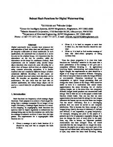
k Fig. 1.

Crossover error probabilities for minimum length linear codes.

(p) is

(2m + 2(2m − 1)

p 1−p

(7)

p2 ) + (2 − 1)(2 − 2) (1 − p)2 m

H5

0.1

m

Table I gives the crossover error probabilities where the first few Hamming codes become better than projection. Theorem 4: For any m > 4 and p > m/(2m − m), the Hamming code Hm beats (2m − m − 1)-projection. Proof: The difference between the distribution functions of the cube and the 1-sphere in dimension 2m − 1 is fm (ζ) := A(S, ζ) − A(Hm , ζ) = 2m (1 + ζ)m

(8)

−(2m + 2(2m − 1)ζ + (2m − 1)(2m − 2)ζ 2 ). We will show that, for m ≥ 4, fm (ζ) has exactly one root in (0, 1), denoted by αm , and that αm ∈ ((m − 2)/2m , m/2m ). We calculate fm (ζ) = ((m − 2)2m + 1)ζ      m 2m m − 2 − 3+ 2 + 2 ζ2 2 m   X m i m ζ . +2 i i=3 All the coefficients of fm (ζ) are non-negative with the exception of the coefficient of ζ 2 , which is negative for m ≥ 2. Thus, by Descartes’ rule of signs f (ζ) has 0 or 2 positive roots. However, it has a root at ζ = 1. Call the other positive root αm . We have fm (0) = fm (1) = 0, and since f ′ (0) = (m−2)2m +2 > 0 and f ′ (1) = 22m−1 (m−4)+2m+2 −2 > 0 for m ≥ 4, we must have αm < 1 for m ≥ 4. For p > αm the Hamming code Hm beats projection. Using (8) and Bernoulli’s inequality, it is easy to show that fm (ζ) > 0 for ζ < c(m − 2)/2m for any c < 1 and m ≥ 4. For the other direction, we may use Taylor’s theorem to show  m m−2 m4  m m < 2m + m2 + m+1 1 + m . 2m 1 + m 2 2 2 Plugging this into (8), we have that fm (m/2m ) < 0 for m > 6.

D. Other Linear Codes The above codes give hashing strategies for a few values of n and k, but we would like hashes for a wider range. For a hashing strategy using error-correcting codes, we need a code with an efficient complete decoding algorithm; that is a way to map every vector to a codeword. Given a translation invariant decoder, we may determine S, the set of vectors that decode to 0, in order to compare strategies as the error probability changes. Magma [6] has a built-in database of linear codes over F2 of length up to 256. Most of these do not come with efficient complete decoding algorithms, but magma does provide syndrome decoding. Using this database new hashing schemes were found. For each dimension k and minimum distance d, an [n, k, d] binary linear code with minimum length n was chosen for testing.1 (This criterion excludes any codes formed by concatenating with a projection code.) For each code there is an error probability above which the code beats projection. Figure 1 shows these crossover probabilities. Not surprisingly, the [23, 12, 7] Golay code G and Hamming codes H4 and H5 all do well. The facts that concatenating the Golay code with projection beats the chosen code for 13 ≤ k ≤ 17 and concatenating Hm with projection beats the chosen codes for 27 ≤ k ≤ 30 show that factors other than minimum length are important in determining an optimal hashing code. As linear codes are subspaces of Fn2 , lattices are subspaces of Rn . The 24-dimensional Leech lattice is closely related to the Golay code, and also has particularly nice properties. It was used in [2] to construct a good LSH for Rn . III. O PTIMAL S ETS In the previous section we looked at the performances of sets associated with various good error-correcting codes. However, the problem of determining optimal sets S ⊂ Fn2 is of independent interest. The general question of finding an optimal set of size 2t in V for an error probability p is quite hard. In this section we will find the answer for t ≤ 6, and look at what happens when p is near 1/2. 1 The

magma call BLLC(GF(2),k,d) was used to choose a code.

4

A. Optimal Sets of Small Size

We have

For a vector x = (x1 , . . . , xn ) ∈ V, let ri (x) be x with the i-th coordinate complemented, and let sij (x) be x with the i-th and j-th coordinates switched. Definition 5: Two sets are isomorphic if one can be gotten from the other by a series of ri and sij transformations. Lemma 6: If S and S ′ are isomorphic, then PS (p) = PS ′ (p) for all p ∈ [0, 1]. The corresponding non-invertible transformation are: ρi (x) := (x1 , x2 , . . . , xi−1 , 0, xi+1 , . . . xn ) ,  x, xmin(i,j) = 0, σij (x) := sij (x), xmin(i,j) = 1.

(9)

Definition 7: A set S ⊂ V is a down-set if ρi (S) ⊂ S for all i ≤ n. Definition 8: A set S ⊂ V is right-shifted if σij (S) ⊂ S for all i, j ≤ n. Theorem 9: If a set S is optimal, then it is isomorphic to a right-shifted down-set. Proof: We will show that any optimal set is isomorphic to a right-shifted set. The proof that it must be isomorphic to a down-set as well is similar. A similar proof for distance-sum optimal sets (see Section III-B) was given by K¨undgen in [18]. Recall that (1 − p)n X d(x,y) PS (p) = ζ , |S| x,y∈S

where ζ = p/(1 − p) ∈ (0, 1). If S is not right-shifted, there is some x ∈ S with xi = 1, xj = 0, and i < j. Let ϕij (S) replace all such sets x with sij (x). We only need to show that this will not decrease PS (p). Consider such an x and any y ∈ S. If yi = yj , then d(x, y) = d(sij (x), y), and PS (p) will not change. If yi = 0 and yj = 1, then d(x, y) = d(sij (x), y) − 2, and since ζ l−2 ≥ ζ l , that term’s contribution to PS (p) increases. Suppose yi = 1 and yj = 0. If sij (y) ∈ S, then d(x, y) + d(x, sij (y)) = d(sij (x), y) + d(sij (x), sij (y)), and PS (p) is unchanged. Otherwise, ϕij (S) will replace y by sij (y), and d(x, y) = d(sij (x), sij (y)) means that PS (p) will again be unchanged. Let Rs,n denote an optimal set of size s in Fn2 . By computing all right-shifted down-sets of size 2t , for t ≤ 6, we have the following result: Theorem 10: The optimal sets R2t ,n for t ∈ {1, . . . , 6} correspond to Tables IV [pg. 7] and V [pg. 8]. These figures, and details of the computations, are given the Appendix. Some of the optimal sets for t = 6 do better than the sets corresponding to the codes in Figure 1. B. Optimal Sets for Large Error Probabilities Theorem 1 states that for any n and k, for a sufficiently small error probability p, a 2n−k -subcube is an optimal set. One may also ask what an optimal set is at the other extreme, a large error probability. In this section we use existing results about minimum average distance subsets to list additional sets that are optimal as p → 1/2−.

  p (1 − p)n A S, |S| 1−p 1 X = Ai pi (1 − p)n−i . i |S|

PS (p) :=

Letting p = 1/2 − ε and s = |S|, PS (γ) becomes X i n−i s−1 Ai (1/2 − ε) (1/2 + ε) i X   1 X 2 A + ε + O(ε ) 2(n − 2i)A = i i i i s 2n s 4ε X = n (1 + 2nε) − n iAi + O(ε2 ) . i 2 s2 Therefore, an optimal set for p → 1/2− must minimize the distance-sum of S 1X 1 X d(x, y) = iAi . (10) d(S) := i 2 2 x,y∈S

Denote the minimal distance sum by f (s, n) := min {d(S) : S ⊂ Fn2 , |S| = s} . If d(S) = f (s, n) for a set S of size s, we say that S is distance-sum optimal. The question of which sets are distancesum optimal was proposed by Ahlswede and Katona in 1977; see K¨undgen [18] for references and recent results. This question is also difficult. K¨undgen presents distancesum optimal sets for small s and n, which include the ones of size 16 from Table IV. Jaeger et al. [15] found the distancesum optimal set for n large. Theorem 11: (Jaeger, et al. [15], cf. [18, pg. 151]) For n ≥ s − 1, a generalized 1-sphere (with s points) is distancesum optimal unless s ∈ {4, 8} (in which case the subcube is optimal). From this we have: Corollary 12: For n ≥ 2t − 1, with t ≥ 4 and p sufficiently close to 1/2, a (2t − 1)-dimensional 1-sphere is hashing optimal. IV. H ASHES

FROM

R ANDOM C ODES

In this section we will show that hashes from random codes under minimum weight decoding2 perform better than projection. Let R = k/n be the rate of a code. The error exponent for k-projection, E Pn,k (p), is 1 1 lg P n,k (p) = − lg(1 − p)k = −R lg(1 − p). (11) n n Theorem 4 shows that for any p > 0 there are codes with rate R ≈ 1 which beat projection. For any fixed R, we will bound the expected error exponent for a random code R of rate R, and show that it beats (11). Let H be the binary entropy −

H(δ) := −δ lg δ − (1 − δ) lg(1 − δ) .

(12)

Fix δ ∈ [0, 1/2). Let d := ⌊δn⌋, let Sd (x) denote the sphere of radius d around x, and let V (d) := |Sd (x)|. 2 Ties arising in minimum weight decoding are broken in some unspecified manner.

5

It is elementary to show (see [11], Exercise 5.9): Lemma 13: Let R be a random code of length n and rate R, where n is sufficiently large. For c ∈ R, the probability that a given vector x ∈ Sd (c) is closer to another codeword than c is at most 2n(H(δ)−1+R) . Lemma 13 implies that if H(δ) < 1 − R (the GilbertVarshamov bound), then with high probability, any given x ∈ Sd (c) will be decoded to c. For the rest of this section we will assume this bound, so that Lemma 13 applies. Let PR (p) be the probability that a random point x and x + e both hash to c. This is greater than the probability that x + e has weight exactly d, so  d   X d n − d 2i p (1 − p)n−2i . PR (p) > i i i=0 Theorem 4 of [3] gives a bound for this: Theorem 14: For any ε ≤ 1/2 and δ such that H(δ) < 1 − R and ε ≤ 2δ, −ER (p) ≥ ε lg p + (1 − ε) lg(1 − p)   ε ε + δH + (1 − δ)H 2δ 2(1 − δ) for any ε ≤ 1/2. The right hand side is maximized at εmax satisfying (2δ − εmax )(2(1 − δ) − εmax ) (1 − p)2 = . 2 εmax p2 Define ε D(p, δ, ε) := ε lg p + (1 − ε) lg(1 − p) + δH 2δ   ε + (1 − δ)H 2(1 − δ) − (1 − H(δ)) lg(1 − p) . Then E Pn,k (p) − ER (p) ≥ D(p, δ, ε). Theorem 15: D(p, δ, εmax ) > 0 for any δ, p ∈ (0, 1/2). Proof: Fix δ ∈ (0, 1/2), and let f (p) := D(p, δ, εmax ). It is easy to check that: lim f (p) = 0,

p→0+

lim f (p) = 0,

p→1/2− ′

lim f (p) > 0,

p→0+

lim f ′ (p) < 0,

p→1/2−

Therefore, it suffices to show that f ′ (p) has only one zero in (0, 1/2). Observe that εmax is chosen so that ∂D ∂ε (δ, p, εmax ) = 0. Hence ∂D (δ, p, εmax) f ′ (p) = ∂p 1 − εmax 1 − H(δ) εmax − + , = p log(2) (1 − p) lg(2) (1 − p) log(2) so εmax 1 − εmax 1 − H(δ) log(2)f ′ (p) = − + . p 1−p 1−p

Therefore f ′ (p) = 0 when εmax = pH(δ). From Theorem 14 we find 4δ(1 − δ) − H(δ)2 p= . 2(H(δ) − H(δ)2 ) Thus we have E Pn,k (p) > ER (p), and so: Corollary 16: For any p ∈ (0, 1/2), R ∈ (0, 1) and n sufficiently large, the expected probability of collision for a random code of rate R is higher than projection. ACKNOWLEDGEMENTS . The authors would like to thank William Bradley, David desJardins and David Moulton for stimulating discussions which helped initiate this work. Also, Tom Dorsey and Amit Khetan provided the simpler proof of Theorem 15 given here. The anonymous referees made a number of good suggestions that improved the paper, particularly the exposition in the introduction. A PPENDIX By Theorem 9, we may find all optimal sets by examining all right-shifted down-sets. Right-shifted down-sets correspond to ideals in the poset whose elements are in Fn2 and with partial order x  y if x can be obtained from y by a series of ρi (9) and σij (10) operations. It turns out that there are not too many such ideals, and they may be computed efficiently. Our method for producing the ideals is not new, but since the main references are unpublished, we describe them briefly here. In Section 4.12.2 of [19], Ruskey describes a procedure GenIdeal for listing the ideals in a poset P. Let ↓x denote all the elements  x, and ↑x denote all the elements  x. procedure GenIdeal(Q: Poset, I: Ideal) local x: PosetElement begin if Q = φ then PrintIt(I); else x := some element in Q; GenIdeal(Q − ↓x, I ∪ ↓x); GenIdeal(Q − ↑x, I); end The idea is to start with I empty, and Q = P. Then for each x, an ideal either contains x, in which case it will be found by the first call to GenIdeal, or it does not, in which case the second call will find it. Finding ↑x and ↓x may be done efficiently if we precompute two |P| × |P| incidence matrices representing these sets for each element of P. This precomputation takes time O(|P|2 ), and then the time per ideal is O(|P|). This is independent of the choice of x. Squire (see [19] for details) realized that, by picking x to be the middle element of Q in some linear extension, the time per ideal can be shown to be O(lg |P|). We are only interested in down-sets that are right-shifted and also are of fairly small size. The feasibility of our computations involves both issues. In particular, within GenIdeal we may restrict to x ∈ Fn2 with Size(↓x) no more than the target size of the set we are looking for. If we were using

6

TABLE II N UMBER OF RIGHT- SHIFTED DOWN - SETS

size 2 3 4 5 6 7 8 9 10

size 11 12 13 14 15 16 17 18 19 20

number 1 1 2 2 3 4 6 7 10

number 13 18 23 31 40 54 69 91 118 155

size 21 22 23 24 32 48 64

number 199 260 334 433 3140 130979 4384627

TABLE III O PTIMAL RIGHT- SHIFTED DOWN - SETS R64,n

BEATING KNOWN CODES .

(T HERE ARE NO SUCH DOWN - SETS R2t ,n k 6 7 8 9 16 17 18 19 20 21

n 12 13 14 15 22 23 24 25 26 27

cross 0.487 0.470 0.439 0.391 0.244 0.242 0.238 0.231 0.222 0.212

FOR

t ≤ 5.)

R64,n h211 , 210 + 25 , 3 · 28 i h212 , 210 + 24 , 3 · 28 i h213 + 22 , 213 + 3, 23 + 22 + 1i h214 + 3, 210 + 22 i h221 + 2i h222 + 1, 219 + 2i h223 + 1, 217 + 2i h224 + 1, 215 + 2i h225 + 1, 213 + 2i h226 + 1, 211 + 2i

GenIdeal with the poset whose ideals correspond to downsets of size 64 in F63 2 , there would be 83, 278, 001 such x to consider. However, for our situation with right-shifted downsets, there are only 257 such x and the problem becomes quite manageable. Furthermore, instead of stopping when Q is empty, we stop when I is at or above the desired size. Table II gives the number of right-shifted down-sets of different sizes. The computation for size 32 sets took just over a second on one processor of an HP Superdome. Size 64 sets took 23 minutes. Let Rs,n refer to an optimal set of size s in Fn2 . Tables IV and V list R2t ,n for all t ≤ 6 and all n < 2t . Several features of Tables IV and V requirePexplanation. i First we identify the binary expansion x = i