the study was to accomplish three objectives: (1) Develop a special online data ...
In a computer adaptive test (CAT), however, the focus is to detect if there is any ...
Online Calibration and Scale Stability of a CAT Program
Fanmin Guo Lin Wang Educational Testing Service, Princeton, New Jersey
Paper presented at the annual meeting of the American Educational Research Association (AERA) and the National Council on Measurement in Education (NCME) held between April 21 to 25, 2003, in Chicago, IL.
Unpublished Work Copyright © 2003 by Educational Testing Service. All Rights Reserved.
These materials are an unpublished, proprietary work of ETS. Any limited distribution shall not constitute publication. This work may not be reproduced or distributed to third parties without ETS's prior written consent. Submit all requests through www.ets.org/legal/copyright
Abstract
This study demonstrates design and analysis methods to evaluate the scale stability of a CAT program using data from a large-scale operational CAT program. The study investigated the calibration and scaling of test items that were pretested online. Using both real and simulated data, the study was to accomplish three objectives: (1) Develop a special online data collection method to study the scale stability, (2) Use test characteristic curves (TCC) and individual item characteristic curves (ICC) to evaluate the stability of a scale by comparing online calibration results at the different time points, and (3) Explore potential impact of scale drift on test scores. Real CAT data were used to yield a realistic ability distribution for simulations. A set of 31 studied items was linearly administered at two time points about 20 months apart and the item parameters were used in simulation. Bias and score impact were evaluated using the observed and simulated scores. The findings from this particular CAT program indicated good scale stability, although small amounts of bias and score impact were detected. The design and methods in this study can be used in CAT programs to monitor scale stability over time.
i
Online Calibration And Scale Stability Of A CAT Program Introduction A stable score reporting scale is the basis for comparing scores from different test administrations. For a testing program that has multiple administrations per year over many years, it is essential that its scale be stable. Special studies are conducted from time to time to monitor the stability of a scale. In a traditional paper-pencil test (PPT), the focus of a scale stability study is to identify scale drift as a result of equating a new test form to ‘one or more of the existing forms for which conversions to the reference scale (i.e., the reporting scale) are already available’ (Angoff, 1984, p. viii). In a computer adaptive test (CAT), however, the focus is to detect if there is any scale drift resulting from errors in the process of item calibration and parameter scaling of new items over time. This is because CAT operates within the framework of item response theory (IRT) and employs some online item calibration method to calibrate and scale new items (Glas, 1998). In IRT, examinees’ ability estimates and item parameters share the same scale, called the θ scale by convention. In an online item calibration design, new items can be linearly administered together with operational items and are calibrated and scaled such that the new items are put on the existing scale of the operational items. Biases and errors in a calibration and scaling process may lead to certain degrees of scale drift over time, and this, in turn, may impact the test scores to the extent that scores may not even be comparable in the worst scenario. In a CAT program, new items are developed, calibrated, and added to an item bank from time to time, and old items are retired due to over the exposure limit or other reasons. Although efforts have been made to calibrate new items and put them on the same scale with the operational items, there is no guarantee that the same scale can be really kept 1
unchanged over a long period of time. In fact, accumulated errors in the calibration and scaling process may lead to changes in a scale. If the scale changes, the original interpretation of scores may no longer be valid. Therefore, it is very important to monitor this in a CAT program. A lot of research has been conducted on equating methods for PPT (Kolen & Brennan, 1995). In CAT, we have found only one directly related reference by Stocking (1988). In this study, Stocking conducted a sequence of six rounds (Round 0 to Round 5) of simulations for online calibration in a CAT environment. All the data were simulated and the researcher did find some evidence of scale drift. Other than this reference, none has been found so far in the educational measurement literature that addresses this important issue of scale stability with online item calibration in operational CAT programs. Moreover, no observed data have ever been used in such a study. As the advance of technology is leading to more CAT programs, it is very important to call attention to scale stability in CAT programs and to design appropriate research to monitor and control scale stability in CAT programs by using both simulations and, more importantly, observed data from live CAT administrations. This was the very intent of designing and conducting this study. The purpose of this study was to demonstrate design and analysis methods to examine the scale stability of a large-scale operational CAT program by investigating the calibration and scaling of test items that were pretested online. Specifically, using both real and simulated data, the study was to accomplish three objectives: (1) Develop a special online data collection method to study the scale stability, (2) Use test characteristic curves (TCC) and individual item characteristic curves (ICC) to evaluate the stability of a scale by comparing online calibration results at the different time points, and (3) Explore potential impact of scale drift on test scores.
2
Methods Investigating the scale stability of a CAT program has two essential foci of interest. One focus is on evaluating item parameters of a group of items that are calibrated and scaled using online pretesting data collected at different time points (for example at Time Point One, or T1, and Time Point Two, or T2). This is like taking one snapshot of the item performance with regard to a reference θ scale at each time point (T1 and T2). When the items are administered linearly and calibrated in the same manner at both administrations, and little change in the item parameters is observed at T1 and T2, we take this as the evidence of the scale stability. The other focus is on possible impact on reported scores if a certain degree of change (scale drift) in item parameters is observed. Because changes in the scale will be reflected in the item parameters derived at T2, any impact of scale drift on test scores will also be observed at T2 when the item parameters at T2 are used in estimating examinees’ ability on the θ scale. Accordingly, this study was designed to investigate these two foci of interest in the following two parts. Figure 1 is a flowchart depicting the major steps of this study. Insert Figure 1 about here.
Part 1-Evaluating scale stability with observed (real) data. Data. Real CAT data were collected from two live administrations of a large-scale CAT program at T1 and T2 because we want to know whether there is any change in the item parameters between T1 and T2 when the items were administered in operational situations. Thirty-one studied items were selected and used in this study. These 31 items were administered linearly together with CAT operational items at both T1 and T2 about 20 months apart. This 20-month interval was chosen according to the testing cycles of the CAT program. After each administration, the items 3
were calibrated in PARSCALE (The ETS internal version of Muraki & Bock, 1999) with the operational items. In the calibration, an item specific prior method (Folk & Golub-Smith, 1996; Guo, Stone, & Cruz, 2001) was used to keep both calibrations on the same θ scale that is used for scoring in this CAT program. Analysis. Differences between the two sets of item parameters at T1 and T2 were evaluated, both individually and collectively. For each item at each time point, an ICC was constructed by calculating the item’s conditional probability, P(Xi = 1 |θ, ai, bi, ci), where θ = -4, -3.9, … 0 … 3.9, 4, and a, b, c are item parameters, over all the 81 points between –4 and 4 on the θ scale. Using these 81 points with an interval of only 0.1 on the θ scale yields more accurate results than using only 20 or 40 points. The difference between the two sets of probabilities, PT1 and PT2, is evaluated using a root mean squared difference (RMSD) method: 4
RMSDICC =
∑ ( Pθ θ = −4
,T 2
− Pθ ,T 1 ) 2
81
(1)
Since RMSD is based on differences between two probabilities, RMSD statistics range from 0 to 1, with smaller values indicating smaller differences. A TCC was constructed at T1 and T2 using the sum of all the item probability (ICCs) over the 81 points on the θ scale. The difference between two TCCs at T1 and T2 can also be evaluated with a RMSD: 4
RMSDTCC =
∑ (τθ θ = −4
,T 2
− τ θ ,T 1 ) 2
81
(2)
k
where τ = ∑ Pθ for the k items of a measure. However, this RMSD range from 0 to τ, the i =1
total number correct score, which is also the same as the total number of items in the measure. To 4
put this RMSD to the same scale of 0 to 1 as for the ICCs, we need to change τ, a total right value, to p*, a proportion of correct value in the Formula (2) above, where p* = τ / k. Therefore, we have: 4
RMSDTCC =
∑ (P θ θ *
,T 2
− P*θ ,T 1 ) 2
= −4
81
(3)
This is what we used for TCC RMSD statistics for the two measures. Part 2-Evaluating score impact with simulation data.
Simulation is a powerful and practical means of investigation that is extensively used in CAT research and operations. A typical simulation involves using true values of both item parameters and simulee abilities (from some assumed distribution such as an uniform or a normal distribution) to generate simulees' responses by administering the items to the simulees. Then the simulees' abilities and/or item parameters are estimated from the simulated data and are compared. Data generation. In this study, to be as close to the reality of the CAT program as possible,
we decided to use the actual ability estimates of all test-takers in a testing year of the CAT program as the true abilities instead of sampling from any assumed typical distribution. We use T0 to indicate the time point for the original ability estimates from the observed data. For each theta at T0 that was treated as an examinee’s true ability value θj, one vector (string) of item responses (1s and 0s) was generated using the item parameters from T1. This process simulates the performance of the examinees taking a linear test with the 31 items at T1. The method of generating a response of 1 or 0 involved comparing a probability value, Pran, that was randomly taken from a uniform distribution with the probability (Pj) of a correct response by the jth simulee given this examinee’s true ability θj and the administered items’ parameters. The response is 0 if Pran is greater than Pj, or 1 otherwise.
5
Using the item responses from the generating θj and the item parameters at T1, a maximum likelihood estimate (MLE) was computed as the theta estimate θ� (j,T1). These new theta values were then converted to scale scores, SS(j,T1) for this jth simulee. To figure out the degree of impact on test scores due to changes in item parameters over time, we need to fix the item responses at both T1 and T2 to simulate the same test performance at these two time points. Therefore, we used the same item responses that were generated at T1 and the item parameters from T2 to calculate the MLEs for the theta estimates at T2, θ� (j,T2), and then converted the theta values to scale scores, SS(j,T2). Each simulated test-taker now has three theta scores: θ(j,T0), (this is the observed theta used as the true theta), θ� (j,T1), and θ� (j,T2), and three scale scores: SS(j,T0) (this is the observed scale score of each examinee), SS(j,T1), and SS(j,T2). Aanalysis. As the conversion of thetas to scale scores is not linear, the impact of scale drift
in theta units might be different from that in the scale score units. In this study, we evaluated the score impact in the scale score units because the scale score is the reporting score. Differences between SST0 and SST1 is in essence an estimate of bias, which by definition is a difference between a true value and an estimate of the true value. On the other hand, differences between SST1 and SST2 are an estimate of score impact due to scale drift: Bias = SST1 - SST0 Impact = SST2 - SST1 Since SST1 and SST2 scores are from theta values that were estimated from the same set of item responses but two sets of item parameters, any differences between SST1 and SST2 can only be attributed to the differences in the two sets of item parameters that are used to obtain these two
6
scores. These differences represent score impact due to scale drift. On the other hand, if the scale of the CAT program is stable, we expect to see little difference between SST1 and SST2. We examined both the overall score impact and conditional score impact for different ability ranges. The overall score impact looks at possible impact over the entire ability scale. However, such score impact may not distribute uniformly across the entire ability scale. More likely, the impact may vary along the ability scale. Therefore, it is necessary and important to examine score impact at different ability levels or within several ability ranges. To be practical for this study, we divided the test-takers into four quarters of ability groups, Q1 to Q4, by their original scale scores (SST0), ranging from 0 to 45. Table 1 specifies the score ranges for each ability level. Both bias and impact were analyzed for each ability group. Insert Table 1 about here.
Results and discussions Part 1. Evaluating scale stability with real data.
The distribution of the RMSD of ICCs for the 31 items is summarized in Table 2, and portrayed in Figure 2. As was mentioned earlier, the RMSD statistic is on a scale of 0 to 1 when a difference is between two probabilities. In item evaluation where probabilities or proportions are compared, 0.05 is typically used as a rule-of-thumb criterion. If a RMSD value is less than 0.05, the difference is considered acceptable for practical purposes. Table 2 shows that the mean RMSD is 0.036 and the median is 0.023, indicating that, on average, there is very little difference in the ICCs between T1 and T2. In other words, average item performance shows little change or drift from the first administration T1 to the second one at T2.
7
Insert Table 2 about here.
When we look at individual item’s RMSD in Figure 2, we find three items with RMSD larger than 0.05. Of the three, only one is above 0.07, while the other two are just above 0.5. Therefore, most of the items demonstrate very similar performance over the span of 20 months, and the scale remains stable over the time. Insert Figure 2 about here.
Because we are more interested in the performance of a test than an individual item, it is necessary to see how the entire test of the 31 items performed at two time points. This evaluation is done using the TCCs and the RMSD that is based on the TCC scales. The RMSD calculated with Formula (3) for the TCCs at T1 and T2 is 0.00842, which is much smaller than our criterion of 0.05 and indicates very little difference between the two TCCs. This finding is also apparent in Figure 3, which displays the TCCs of T1 and T2. The vertical axis gives the expected number correct scores k
( τ = ∑ Pθ ), ranging from 0 to 31. The horizontal axis shows the θ scale with selected points of i =1
equal intervals. The solid line is for T1 and the dotted line is for T2. The two lines are very close to each other across the entire θ scale, with T1 slightly lower than T2 between θ = -0.2 and θ = 3. This indicates that the test was slightly harder at T1 than at T2, the difference is, however, too small to be of practical significance. In short, the findings from both the individual item level and the test level show very small differences in the performance of the items between T1 and T2. These findings provide good evidence that the scale remained stable for the time period of interest in this study. 8
Insert Figures 3 and 4 about here.
Part 2. Evaluating scale impact with simulation data.
Table 3 presents the summary statistics of the scale scores for both the simulated and real data. The real data scores are treated as true scores and are denoted as SST0. The scores from the simulation data are indexed as SST1 and SST2, respectively. The minimum and maximum values show the score ranges. It appears that the mean scores are slightly lower from SSTO (30.01) through SST1 (29.95) to SST2 (29.37). The change is, however, less than a score point on the 46-point scale. The mean socre of SST1 is smaller than that of SST0, the difference between the two is rounded to – 0.06 (see the cell of Overall and Bias in Table 4). The difference is about - 0.13% of the possible 46 score points (see Table 5). As was mentioned before and is indicated in the column headings in Tables 4 and 5, this –0.06 or –0.13% difference between SST1 and SST0 (SST1 - SST0) is defined as an estimate of bias. This small amount of negative bias suggests that the average ability of the simulated sample is slightly lower than that of the sample of true ability. However, the bias is very small and is trivial in a practical sense. Insert Tables 3, 4, and 5 about here.
The score impact estimate for the overall sample is the difference between SST2 and SST1, or SST2 - SST1. The difference is – 0.58 with a standard deviation of 0.695 (Table 4). Similarly, this different is translated to – 1.29% of the score range in Table 5. The negative impact value of – 0.581 indicates that, on average, the same test takers at T2 would score slightly over half a point lower than at T1 on exactly the same test. This result is in agreement with the TCC chart of Figure 3. The TCCs at T1 (solid line) and T2 (dotted line) displays a slight gap over an interval of 9
theta scale, suggesting that the same test (same items but different item parameters for T1 and T2) appears to be slightly easier at T2 than at T1. Because the simulation data were generated from the true ability score (θT0) and the item parameters at T1, and the items are harder at T1 than at T2, it follows that the ability estimates from the same responses have to be lower at T2 than at T1. At the four different ability levels (Q1 – Q4) in Tables 3 and 4, we see that the estimated bias goes from – 0.04 (or – 0.09%) at Q3 to – 0.27 (- 0.59%) at Q4. The bias is negative at all levels except Q2, where the bias estimate is 0.20 or 0.44%. Again, all these bias values are very small, the largest being only slightly higher than half a percent (Q4). Therefore, the bias values for the four ability levels can be ignored. The score impact spreads between – 0.40 (Q4) and – 0.74 (Q3), and is negative for all levels. The largest difference is close to one score point, or 0.64% of the score range at Q3. Relatively speaking, the score impact is observed to be greater at Q2 and Q3 than elsewhere on the ability scale, although the absolute bias is small across the board. In summary, bias and score impact were found, but the degrees of bias and impact vary in a number of ways. Figure 4 presents a view of the distributions of the bias and impact by ability level (note that the vertical axis is reversed so that the negative values are at the top portion of the chart). It is apparent that bias is very small across the board and it is practical to ignore the presence of such trivial amount of bias in the current data. Insert Figure 4 about here.
Conclusions
Score comparability is a major concern for a testing program in terms of both content and measurement precision (Kolen, 1999-2000; Wang & Kolen, 2001). The issue of scale stability in this study is a special aspect of score comparability in a CAT program, which has largely been 10
explored. This study was to draw attention to this issue and to obtain a preliminary understanding of what scale drift may bring about to a CAT program. The findings from the analyses of the real data at the two time points found very little changes in the TCCs at T1 and T2, although a few individual items did exhibit slightly greater changes than other items. These findings give some assurance about the stability of the scales that are used in the CAT program under this study. The results from the simulation part of the study demonstrated how changes in the scale would impact ability estimation and test scores. For example, the tests were slightly easier at T2 than T1 (as shown in TCCs in Figure 3), as a result, an ability estimate using the same responses would become lower at T2 than T1. For this study, because the changes in the TCCs were very small, the score impact was accordingly small and was considered practically nonsignificant. However, it is, not difficult to infer what score impact would look like if sizable scale drift is present. When this happens, the measurement precision is no doubt different at two time points, and some scale adjustment is then urgently required to support score comparability at T1 and T2. This study used one CAT program and two time points only in investigating scale stability over time. Nevertheless, the methods for data collection, simulation setup, and analyses can be readily applied to studying this issue with other CAT operational programs. We hope to see more research in this area, either in similar studies as ours or by developing new methods of inquiry.
11
References
Angoff, W. H. (1984). Scales, norms, and equivalent scores. Princeton, NJ: Educational Testing Service. Glas, C. A. W. (1998). Quality Control of On-Line Calibration in Computerized Assessment. (Research Report 98-03). The Netherlands: University of Twente. Folk, V. & Golub-Smith, M. (1996) Calibration of on-line pretest data using BILOG. Paper presented at the annual meeting of NCME, Chicago. Guo, F. Stone, E. & Cruz, D. (2001). On-line Calibration Using PARSCALE Item Specific Prior Method: Changing Test Population and Sample Size. Paper presented at NCME Annual
Meeting, Seattle, Washington. Kolen, M. J. (1999-2000). Threats to score comparability with applications to performance assessments and computerized adaptive tests. Educational Assessment, 6(2), 73-96. Kolen, M. J., & Brennan, R. L. (1995). Test equating methods and practices. New York: SpringerVerlag. Muraki, E. & Bock R. (1999). PARSCALE 3.5: IRT item analysis and test scoring for rating-scale
data. Scientific Software, Inc. Stocking, M. (1988). Scale drift on-line calibration. (ETS Research Report 88-28-ONR). Princeton, NJ: Educational Testing Service. Wang, T., & Kolen, M. J. (2001). Evaluating comparability in computerized adaptive testing: Issues, criteria and an example. Journal of Educational Measurement, 38(1), 19-49.
12
Table 1. Score ranges for the four ability levels Quartile Q1 Q2 Scale Scores (T0) 0 - 23 24 - 31
Q3 32 - 38
Q4 39 - 45
Table 2. Summary statistics for RMSD between ICCs of T1 and T2. Standard N Mean Median Minimum deviation 31 0.036 0.015 0.023 0.009
Table 3. Summary statistics of the scale scores of the real and simulated data. Score N Mean Std. Dev. Minimum Maximum SST0
169111
30.01
10.283
0
45
SST1
169111
29.95
10.830
0
45
SST2
169111
29.37
10.806
0
45
Table 4. Summary information of the estimated bias and impact. Group Overall Q1 Q2 Q3 Bias Mean -0.06 -0.13 0.2 -0.04 Std. Dev. 3.601 4.461 3.828 3.567 Impact Mean -0.58 -0.48 -0.72 -0.74 Std. Dev. 0.695 0.812 0.667 0.64
Q4 -0.27 1.979 -0.4 0.556
Table 5. Bias and impact estimates in percentage of scale score range Overall Q1 Q2 Q3 Bias -0.13% -0.28% 0.43% -0.09% Impact -1.26% -1.05% -1.57% -1.60%
Q4 -0.58% -0.87%
13
Maxmum 0.075
Figure 1. Flowchart of the Study Part 1
Studied items Data collection, calibration & scaling (T2)
Data collection, calibration & scaling (T1) Item parameters (T1)
Comparing TCCs & ICCs
Item parameters (T2)
Observed examinees' theta (T0)
Part 2
Simulation Simulees' responses Scoring & conversion (T1) Simulees' scores (T1)
Scoring & conversion (T2) Comparing simulees' scores
14
Simulees' scores (T2)
Figure 2. RMSD between T1 and T2 ICCs 0.08
0.07
0.06
0.05
0.04
0.03
0.02
0.01
0.00 1
2
3
4
5
6
7
8
9
10
11
12
13
14
15
16
17
18
19
2
21
2
2
2
2
2
2
2
2
3
31
It em
Figure 3. TCCs of T1 and T2 35 30
T1
Total Right
25
T2
20 15 10 5 0 -4
-3.5
-3
-2.5
-2
-1.5
-1
-0.5
0
0.5
Theta
15
1
1.5
2
2.5
3
3.5
4
Figure 4. Bias and impact by ability -2.00
Bias Impact
-1.50
Percent
-1.00
-0.50
Overall
Q1
Q2
0.00
0.50
16
Q3
Q4