Online Defect Prediction for Imbalanced Data - CiteSeerX

Online Defect Prediction for Imbalanced Data Ming Tan

Lin Tan

Sashank Dara

Caleb Mayeux

University of Waterloo, Canada [email protected]

University of Waterloo, Canada [email protected]

Cisco Systems, India [email protected]

Cisco Systems, USA [email protected]

Abstract—Many defect prediction techniques are proposed to improve software reliability. Change classification predicts defects at the change level, where a change is the modifications to one file in a commit. In this paper, we conduct the first study of applying change classification in practice. We identify two issues in the prediction process, both of which contribute to the low prediction performance. First, the data are imbalanced—there are much fewer buggy changes than clean changes. Second, the commonly used cross-validation approach is inappropriate for evaluating the performance of change classification. To address these challenges, we apply and adapt online change classification, resampling, and updatable classification techniques to improve the classification performance. We perform the improved change classification techniques on one proprietary and six open source projects. Our results show that these techniques improve the precision of change classification by 12.2-89.5% or 6.4–34.8 percentage points (pp.) on the seven projects. In addition, we integrate change classification in the development process of the proprietary project. We have learned the following lessons: 1) new solutions are needed to convince developers to use and believe prediction results, and prediction results need to be actionable, 2) new and improved classification algorithms are needed to explain the prediction results, and insensible and unactionable explanations need to be filtered or refined, and 3) new techniques are needed to improve the relatively low precision.

I. I NTRODUCTION Software defect prediction techniques leverage information such as code complexity, code authors and software development history to predict code areas that potentially contain defects [1]–[9]. Code areas that contain defects are also referred to as buggy code areas. Defect prediction techniques typically predict defects in a component [4], [8], [10], [11], a file [3], [7], [12], a method [13], or a change [1], [2], [14], [15]. A change is the committed code in a single file [1]. A recent study [16] reports the experience and lessons learned of predicting buggy files at Google. Compared to file level prediction, the application of change level prediction has its benefits and challenges. Following the prior work [1], we refer to change level prediction as change classification. Change classification [1], [14], [15], [17] can predict whether a change is buggy at the time of the commit, which allows developers to act on the prediction results as soon as a commit is made. In addition, since a change is typically smaller than a file, developers have much less code to examine in order to identify defects. However, for the same reason, it is more difficult to predict on changes accurately. To the best of our knowledge, there are no published case studies of the application of change classification on a

proprietary code base in industry. In this paper, we apply change classification on a proprietary code base at Cisco and share the experience and lessons learned. A high prediction precision is important for the adoption of change classification in practice. If a developer finds that many predicted buggy changes contain no real bugs, i.e., the changes are clean, developers are likely to ignore all prediction results. We apply change classification techniques [17] on one of Cisco’s code bases and adapt them for integration in practice. We find that the precision is only 18.5%, which is significantly lower than the precisions on open source projects [1], [17]. We have identified the following main reasons. 1) The Challenge of Imbalanced Data The proprietary code base has a lower buggy rate—the percentage of changes that are buggy—than that of the open source projects. In other words, the data in the code base are imbalanced. When the buggy rate is low, it is challenging to learn accurate models because there are fewer positive instances (i.e., buggy changes) for learning. Classifying imbalanced data is a known open challenge [18]. Irrespective of proprietary or open source, the data sets are imbalanced. The six evaluated open source projects, Linux kernel, PostgreSQL, Xorg, Eclipse, Lucene, and Jackrabbit, have buggy rates of 14.7–37.4%, whereas the buggy rate of the proprietary project is below 14% (Table I). Thus, solutions to address the imbalanced data challenge should improve the performance, e.g., precision and recall, of change classification on both proprietary and open source projects. To address the imbalanced data challenge, we leverage techniques to increase the percentage of positive instances in the training set. The training set contains the data used to train the model, while the test set contains the data to evaluate the model. For example, a simple resampling technique duplicates positive instances in the training set to balance the two classes. Four resampling approaches, i.e., Simple Duplicate, the Synthetic Minority Oversampling Technique (SMOTE), Spread Subsample, and Resampling with/without Replacements, are used to improve the performance of change classification. The test set is unchanged for an objective evaluation of the classification performance. 2) False High Precisions from Cross-Validation K-fold cross-validation is commonly used to evaluate software defect prediction [1], [6]–[8], [14], [17]. Specifically, k-fold crossvalidation randomly divides a data set into k partitions (k > 1),

c 2015 IEEE. Personal use of this material is permitted. Permission from IEEE must be obtained for all other uses, in any current or future media, including Accepted for publication by IEEE. reprinting/republishing this material for advertising or promotional purposes, creating new collective works, for resale or redistribution to servers or lists, or reuse of any copyrighted component of this work in other works.

and uses k − 1 partitions to train the prediction model and the remaining 1 partition as the test set to evaluate the model. However, cross-validation is inappropriate for estimating the performance of change classification because the data points, i.e., changes, follow a certain order in time. Randomly partitioning the data set may cause a model to use future knowledge which should not be known at the time of prediction to predict changes in the past. For example, cross-validation may use information regarding a change committed in 2014 to predict whether a change committed in 2012 is buggy or clean. This scenario would not be a real case in practice, because at the time of prediction, which is typically soon after the change is committed in 2012 for earlier detection of bugs, the change committed in 2014 is nonexistent yet. Using cross-validation could also cause the data to be labeled ahead by currently unknown data. Section III-A provides the details of these problems. In practice, we need time sensitive change classification. In other words, at time t when a change c is committed, the information used to classify c or any change before c should be information known until time t only. To test the impact of cross-validation, we applied both 10-fold crossvalidation and time sensitive change classification on seven projects (one proprietary and six open source). We found that the precision of time sensitive change classification is only 18.5–59.9%, while the precision of cross-validation is 55.5– 72.0% for the same data (details in Section VI-A). The results suggest that cross-validation presents a false impression of higher precisions. This paper makes the following contributions: •

•

•

We apply and adapt time sensitive change classification and online change classification, both addressing the problems of change classification with cross-validation. We leverage resampling techniques to address the imbalanced data challenge, and apply updatable classification algorithms to improve classification performance as well. These techniques have improved the precision of time sensitive change classification by 12.2-89.5% or 6.4–34.8 percentage points (pp.) on the one proprietary project and six open source projects. If a technique improves the precision from a to b, the technique improves the precision by ((b − a)/a)% or (b − a) pp. We conduct the first case study of integrating change classification in the development process of a proprietary project. In addition to the prediction (whether a change is buggy or not), we generate and improve explanations from prediction models and present them to Cisco developers. Explanations were lacking in previous studies [16], [19], which makes it hard for developers to act on the prediction [16].

The main lessons learned include 1) since change classification is relatively new to developers, we need new solutions to convince developers to use and believe prediction results and make prediction results actionable; 2) new and improved classification algorithms for explaining the prediction results

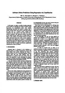
Fig. 1. Process of Change Classification. A check mark annotates a clean change, and a cross mark annotates a buggy change.

are needed, and insensible and unactionable explanations need to be filtered or refined; and 3) even with the improved approaches, the prediction precision is still relatively low, suggesting that new techniques are needed to improve the precision. II. S OFTWARE C HANGE C LASSIFICATION This section provides a background of change classification. Figure 1 shows the process of change classification [1], which consists of the following steps: 1) labeling each change as buggy or clean to indicate whether the change contains bugs; 2) extracting the features to represent the changes; 3) using the features and labels to construct a prediction model; 4) extracting the features for new changes and applying the model to predict their labels. A. Labeling Buggy and Clean Changes The labeling process uses data from the Version Control Systems (VCS) and Bug Tracking Systems (BTS). We follow the same approach used in previous work [17], [20], [21]. A line that is deleted or changed by a bug-fixing change is a faulty line. A bug-fixing change is a change that fixes bugs. The most recent change that introduced the faulty line is considered a buggy change. If a project’s BTS is not well maintained and linked, we consider changes whose commit messages contain the word “fix” bug-fixing changes. If a project’s BTS is well maintained and linked, we consider changes whose commit messages contain a bug report ID bug-fixing changes. Manually verified bug reports are available for Lucene and Jackrabbit [22], which are used in our study for extracting more accurate bug-fixing changes. The blaming or annotating feature of the VCS is used to find the most recent changes that modified the faulty line, which are the buggy changes. We consider the remaining changes as clean changes. B. Extracting Features Features are used to represent the changes for prediction. The types of features are the same as those in previous work [17]: metadata, bag-of-words, and characteristic vectors. We use all the meta features from previous work [17], e.g., commit time and full path. In addition, we add the following features: the added line count per change, the deleted line count per change, the changed line count per change, the added chunk count per change, the deleted chunk count per

change, and the changed chunk count per change. The bagof-words feature is a vector of the count of occurrences of each word in the text. We use the snowBall stemmer [23] to group words of the same root and Weka [24] to obtain the bag-of-words features from both the commit messages and the source code. The characteristic vectors consider the count of the node type in the Abstract Syntax Tree (AST) representation of code. Deckard [25] is used to obtain the characteristic vector features. III. A PPROACHES This section first demonstrates the problems of crossvalidation when used for evaluating change classification in practice (Section III-A). It then describes the time sensitive change classification (Section III-B), followed by its improved version—online change classification (Section III-C). Section III-D and III-E present two approaches to improve the performance of the online change classification. A. Problems of Using Cross-Validation for Evaluating Change Classification Cross-validation is a commonly used method to evaluate the prediction models [1], [7], [8], [14], [17], [26]. The process of 10-fold cross-validation is to 1) separate the data set into 10 partitions randomly; 2) use 1 partition as the test set and the other 9 partitions as the training set; 3) repeat step 2) with a different partition as the test set until all the data have a predicted label; 4) compute the evaluation results through comparison between the predicted labels and the actual labels of the data. This process reduces the bias in the error estimation of classification. Using cross-validation to evaluate change classification has two problems (Figure 2). Changes C1–C10 are committed chronologically, where C1 is the oldest, and C10 is the most recent. Dots denote buggy changes, and circles denote clean changes. An arrow links a buggy change and the corresponding change that fixes the buggy change. For example, C4 fixes the bugs in C3; therefore, C3 is a buggy change. First, cross-validation will use future data for prediction. In this example, 10-fold cross-validation will make each change the test set in each iteration. For example, it will use C2–C10 to predict whether C1 is buggy or not, which does not match a real-world usage scenario where we typically want to make the prediction at the time when C1 is committed and by then C2–C10 are not available yet. Second, cross-validation mislabels changes. Using crossvalidation, changes will be labeled as shown in Figure 2 [1], [14], [17]. For example, C5 will be labeled buggy. However, in practice, when we predict whether C6 is buggy, we would only have information at time tpredict . Therefore, C5 should be clean at time tpredict because C7 was nonexistent at that time. It is incorrect for cross-validation to consider C5 buggy when we predict the label of C6 at time tpredict , because we would not know that C5 is buggy at time tpredict . Due to these issues, it is unclear whether precisions obtained from cross-validation are accurate estimates of precisions of

Fig. 2. Illustrating Problems of Using Cross-Validation to Evaluate Change Classification. Dots are buggy changes, while circles are clean changes.

defect prediction in practice. Our experiments show that crossvalidation provides false high precisions (Section VI-A). B. Time Sensitive Change Classification Time sensitive change classification uses information, known at time t only, to classify change c that is committed at t. For example, in Figure 2, time sensitive change classification predicts at time tpredict for the change C6, i.e., the test set. The changes committed before C6 are the training set, i.e., C1-C5, which is used to build models. However, this method has three limitations. First, in practice, we prefer to predict as soon as changes are committed so that we can examine them to identify bugs earlier. Therefore, the time period of the test set is often short, e.g., a few days or months. However, bugs typically take years to be discovered and fixed [27]–[29]. Therefore, at the prediction time tpredict , many buggy changes in the training set, especially the changes committed close to time tpredict , would not have been found and fixed yet. Therefore, many of these changes in the training set, e.g., C5, will be labeled clean, indicating that the buggy rate in the training set, i.e., 1/5, will be lower than the typical buggy rate, i.e., 2/5, of a project. If the buggy rate of the training set is much different from the buggy rate of the test set, a classification algorithm may fail to learn an accurate model for the test set. Second, the performance of time sensitive change classification depends on the particular data set. For example, if we pick a time period which is right before a release deadline for evaluation, then the changes from this time period may not be representative of the changes from other periods of time. Thus, the prediction performance of this time period may not be representative of the performance of other time periods. Third, if the changes in the test set are committed over a long period of time, many development characteristics, such as the development tasks, the developer experience, and the programming styles, may be different from those of the training set. Therefore, the training set may be too old to build accurate prediction models for the test set. C. Online Change Classification To address the three challenges, we use the balanced online time sensitive change classification, online change classification in short. To address the first challenge, we make the training set more balanced in time sensitive models. Specifically, we leave a gap between the training set and the test set (Figure 3), which allows more time for buggy changes in the training set to be discovered and fixed. For example, the time period between time T 2 and time T 4 is a gap. This way, the

Fig. 3. Online Change Classification.

training set will be more balanced, i.e., the training set will have a higher buggy rate which is consistent with the buggy rate in the test set. A reasonable setup is to make the sum of the gap and the test set, e.g., the duration from time T 2 to T 5, close to typical bug-fixing time—the time from a bug is introduced until it is fixed. Our results show that using a gap of 0.2 year yields an average 14.4 pp. improvement on precision for Jackrabbit and 15.5 pp. for PostgreSQL with 1.0 year’s gap. To address the second and third challenges, we make change classification online, which applies multiple runs of time sensitive change classification, where the training set is constantly updated with new data. For each run, we add to the training set the data immediately following the training set. The performance is the weighted average performance of these runs. Online change classification performs prediction on multiple test sets to minimize the bias from a particular test set. Since the training set is constantly updated, the training set is more likely to have similar characteristics as the test set, hence, to construct more accurate models. Figure 3 illustrates the process of online change classification. Two runs are illustrated. The second run combines the training set in the first run and the data from time T 2 and T 3 (i.e., changes from T 1 to T 3) to form the training set for the second run. In this paper, for simplicity, the duration from T 2 to T 3 is the same as the duration from T 4 to T 5, which is the duration for each test set. However, this duration can be other values for generality. The gap for the second run is T 3 to T 5. More recent changes (between T 5 and T 6) form the test set for the second run. The new prediction time is T 6; thus, changes in the new training set will be labeled using information available at time T 6. D. Resampling As discussed in Section I, data for change classification are typically imbalanced, i.e., the buggy changes are much fewer than the clean changes. The clean changes are referred to as the majority class, and the buggy changes are called the minority class. For software with a lower buggy rate, it is harder for classification algorithms to learn the patterns of the buggy changes. We apply two established approaches to improve the prediction performance on imbalanced data—resampling techniques [30] and updatable classification techniques [31]– [37]. This section describes resampling techniques; and Section III-E describes the updatable classification techniques. Resampling is an effective way to mitigate the effects of imbalanced data in change classification [18], [38]. Different algorithms are used to change the distribution between the

majority class and the minority class. Two main categories of resampling techniques are oversampling and undersampling. Oversampling creates more buggy changes; whereas undersampling eliminates clean changes. We use four types of resampling techniques to predict for the imbalanced data: simple duplicate, SMOTE, spread subsample, and resampling with/without replacements [24]. Simple duplicate and SMOTE are oversampling techniques, while spread subsample is an undersampling technique. Resampling with/without replacements can achieve both. We tune the parameters as illustrated in Section V, and reserve the parameters which contribute to the highest precision. 1) Simple Duplicate: randomly copies instances in the minority class to make the two classes have the same number of instances. Due to the randomness, we run this method five times and calculate the average performance. 2) SMOTE: takes the k (k > 1) nearest neighbors of each buggy change according to the Euclidean distance and replicates the nearest changes. 3) Spread Subsample: adjusts the weight of the two classes by removing the instances in the majority class for balancing the ratio of the two classes, ranging from 1:1–10:1. 4) Resampling with/without Replacements: are bootstrapping based approaches. Resampling with replacement ranks changes according to the estimation error of sampling the original data with replacements; then it adds the replication of higher ranking changes. Resampling without replacements randomly picks instances for either eliminating or duplicating. Due to the randomness, multiple runs of the experiments are conducted. E. Updatable Classification Updatable classification algorithms update the training set incrementally to take advantage of the feedback from each run. Our online change classification updates the training set with the test set but does not take advantage of the feedback from the learning process. Therefore, we apply the updatable models to benefit from the feedback in each run. We experiment with the following updatable learning algorithms: Bayes [31], IBK [32], KStar [33], LogitBoost [34], LWL [35], NNge [36], and SPegasos [37]. We select them because they are based on various basic types of machine learning algorithms, including Naive Bayes (Bayes, LWL), instance-based learning (IBK, KStar), boosting (LogitBoost), nearest-neighbors (NNge), and SVM (SPegasos). IV. A C ASE S TUDY OF I NTEGRATING C HANGE C LASSIFICATION R ESULTS IN S OFTWARE D EVELOPMENT We deploy online change classification in the software development process of the evaluated project at Cisco. The goal is to understand how to generate and present explanations of the prediction results to developers, and how to improve online change classification for its adoption in software development. To achieve this goal better, we conduct a qualitative study instead of a quantitative one.

In addition to predicting on each change as it is committed, it is also beneficial to predict on the changes committed in recent years since bugs typically take years to be discovered and fixed [27], [28]. The recently committed changes may be buggy but have not been detected and fixed yet. Therefore, we apply our prediction models on the changes of the proprietary software made in the last year. Before a developer makes a commit, the developer sends the diffs to the review board, i.e., a new review request is created in the review board. The status of a review request is open, submitted, or discarded. An open review request means the commit is not committed to the repository yet and is still in the review stage; a submitted review request means this request has passed the review stage and the change has been committed to the repository; and a discarded review request is a request that has been abandoned after code review. Discarded reviews are not in the software repository; therefore, we do not use them in our experiments. We predict on open review requests to discover buggy changes before their code review has been completed and predict on submitted review requests to discover committed buggy changes. Change classification is integrated after a developer submits a review request of a commit to the review board (Figure 4). Then our change classification tool automatically obtains the diff file—Patches in Figure 4—of this commit and extracts all the features of the commit. Next, it builds a model from recent changes. This model predicts labels of the changes in the commit. If a change is predicted buggy, our tool automatically generates an explanation of why this change is predicted buggy based on the model; then, our tool pushes the explainable results to the review board. The review board notifies the developers of the results. After examining the suggestions provided by change classification, the developers submit the feedback as whether the suggestion is taken or rejected as well as the corresponding reason. To increase the possibility of a positive adoption experience, we select developers on whose changes our tool can predict accurately. Specifically, we first build independent models for each developer who has made at least 100 buggy changes in this project. Among them, we select seven developers whose model(s) built by either resampling techniques or updatable classification could achieve 100% precision on the test sets (Table IV) for this case study. The test sets contain older changes that have been fixed so that we can compare the predicted labels with the actual labels of changes to measure precision. As a small case study, we start with 30 most recent review requests of each selected developer. If a developer has made fewer than 30 review requests, all of the developer’s review requests are selected for this case study. Since it is easier for developers to examine relatively small changes, we only reported the changes with 50 or fewer lines, to the developers. Totally we have predicted 96 small buggy changes of 39 review requests from the seven developers for the field trial. In our pilot study, we create four review requests regarding 11 changes from one developer and four reviewers.

Fig. 4. The Integration of Change Classification in the Code Review Process.

The above process was considered intrusive in a production environment when integrated with the review board. Later we opt for a less intrusive option: emailing prediction results to the developers who are interested in trying out change classification. We have emailed the prediction results of 85 changes to the remaining six developers. We also have enlisted the predictions in a file and verified their validity with a few developers in an offline process. Due to the relatively small scale of the case study, we focus on discussing our qualitative instead of quantitative results. We share the experience learned in conducting this case study in Section VII. V. E XPERIMENTAL S ETUP A. Evaluated Projects We evaluate the change classification techniques on one proprietary project from Cisco and six open source projects, i.e., Linux, PostgreSQL, Xorg, Eclipse, Lucene, and Jackrabbit. For Xorg and Eclipse, only data from a subdirectory is used, i.e., Xserver and JDT core respectively. Columns “Lang” to “Ch” of Table I show the basics of these projects. The features retrieved are from the source code files1 only. B. Data Selection We select changes in the middle of the software history of a project, because the characteristics of a project may be unstable at the beginning of its history. The most recent changes are excluded because buggy changes in them would not have been found and fixed yet. Note that this is for evaluation only. In practice, we predict on the latest changes so that developers can find bugs in them earlier, which is the experiment that we conducted in our case study (Section IV). The specific time parameters used in online change classification are Start-Gap, Gap, End-Gap, and Update-Time. 1) Start-Gap is the time period at the beginning of a project when changes are excluded from our experiments. 2) Gap, e.g., T 2–T 4 or T 3–T 5 in Figure 3, is the time period between the training set and the test set. Adding such a gap allows enough time for buggy changes in the training set to be discovered by the prediction time (Section III-C). 3) End-Gap is the time period at the end of a project’s data collection, when changes are excluded from our experiments. Typically it is the average time that it takes to discover and fix a bug, i.e., the average bug-fixing time. 1 The files with these extensions are included: .java, .c, .cpp, .cc, .cp, .cxx, .c++, .h, .hpp, .hh, .hp, .hxx and .h++.

TABLE I E VALUATED S OFTWARE . L ANG IS THE PROGRAMMING LANGUAGE USED FOR THE PROJECT. LOC IS LINES OF CODE . F IRST DATE IS THE DATE OF THE FIRST COMMIT OF A PROJECT, WHILE L AST DATE IS THE DATE OF THE LATEST COMMIT. C H IS THE TOTAL NUMBER OF CHANGES FOR EACH PROJECT THROUGH LISTED HISTORY. SG IS THE S TART-G AP. EG IS THE E ND -G AP. UT IS U PDATE -T IME . T HE UNIT FOR THE S TART-G AP, G AP, AND E ND -G AP IS year, AND THE UNIT FOR THE U PDATE -T IS day. Project Proprietary Linux PostgreSQL Xorg Eclipse Lucene Jackrabbit

Lang C C C C Java Java Java

LOC >10M 7.3M 289K 1.1M 1.5M 828K 589K

First Date 2003-xx-xx 2005-04-16 1996-07-09 1999-11-19 2001-06-05 2010-03-17 2004-09-13

Last Date 2014-xx-xx 2010-11-21 2011-01-25 2012-06-28 2012-07-24 2013-01-16 2013-01-14

Ch >100K 429K 89K 46K 73K 76K 61K

4) Update-Time, e.g., T 2–T 3, in Figure 3, is the time period used to update the training set to build a new model. Different time parameters are used for different projects due to their data variance, e.g., length of development history and average bug-fixing time. Initially we follow the previous paper [17] for Start-Gaps, which are three years for most projects. To ensure enough runs of experiments, the average test set size is smaller than one fourth of the total count of experimental changes in each project. In addition, we set the quotient of the total experimental change count of each project divided by the number of runs as the upper bound of average training set size. Gap is the difference between average bugfixing time and test set time period for each project. UpdateTime is the same as the test set duration. Given the constraints, our tool automatically determines the number of runs for each project based on the data’s suitability, i.e., the buggy rate in both the training set and the test set for a run should be above 0%. End-Gap is set depending on the number of runs. If the data sets cannot be determined by one run of the tool, i.e., the parameters or the data sets generated do not satisfy the constraints, the tool will add 1 month to the Start-Gap and try to find the desired data sets again. The specific time parameters for the projects are shown in columns “SG” to “UT” of Table I. The remaining columns show the number of changes in our data sets. Certain information of the proprietary project is kept vague for confidentiality. Column “ExpCh” is the number of changes used for the experiment, i.e., all changes excluding the changes during StartGap and End-Gap. All these experimental changes are used for 10-fold cross-validation. Column “ExpBR” is the ratio of the buggy changes in the experimental changes. For our online change classification, we collect data for the multiple runs from the experimental changes as described above. “TrSize” is the average size of training sets in all runs, while“TSize” is the total number of test instances in all runs combined. “NR” is the number of runs for each project. We conduct an additional experiment on selected top developers because the overall precision of online change classification is low. We want to show that we can achieve higher precision on top developers, following previous work [17]. We rank developers by the total number of bugs in their commit history. We pick the top 10 of the developers on the list; then

SG 5.0 3.0 7.0 5.2 5.0 0.5 3.0

Gap x.xx 0.03 0.20 0.40 0.10 0.10 0.20

EG x.x 2.3 5.9 5.0 6.2 1.5 3.3

UT 365 8 60 100 40 30 60

ExpCh >20,000 10,443 10,810 10,956 9,190 11,106 13,069

ExpBR 5,000 1,608 1,232 1,756 1,367 1,194 1,118

TSize >10,000 6,864 6,824 6,710 6,974 9,333 8,887

NR 3 4 7 6 6 8 10

we select the developers whose changes allow for at least two runs and the precision of the first run is higher than 60%. C. Classification Algorithms and Experiments We use alternating decision tree (ADTree [39]) in Weka [24] as the classification algorithm, since it performs best in previous work [17]. ADTree has two parameters: one is the maximum iteration time, and the other determines the number of paths to search for building the tree. We tune the maximum iteration time of ADTree the same way as previous work [17]; and finally we set 10 as the maximum iteration time. We set the default value, i.e., -3, for the second parameter to search all possible paths to find the best model. After we obtain all the preliminary results from the above setting, we apply the resampling and the updatable classification techniques (Section III). We use Weka [24] for all the resampling and updatable classification techniques except the simple duplicate method because Weka does not have an implementation of it. We experiment with following parameter values of the approaches. We report the highest precision for each project, as high precision is crucial for adoption. The number of nearest neighbors in SMOTE ranges from 2 to 10. The percentage of the minority class duplications is within the range (50, 80, 100, 200, 300, 400, 500). For spread subsample, we select the best among all the ratio between the two classes varying from 1:1–10:1. As such, whether to adjust the total weight of the classes depends on the results. For the resampling with/without replacement method, all the combinations of with/without replacement and original/uniform distribution of input data are used. The output percentage of the sample size is in the same range as the SMOTE range list. After tuning, the updatable classification algorithms choose the following values for different parameters: for the Bayes, we do not uniform the distribution of input data. Both IBK and LWL use the linear nearest neighbor search algorithm; and IBK chooses one nearest neighbor. The global blending percentage in the KStar is set to 20%. The default settings (10 iterations, no internal cross-validation, and reweighting for boosting) are used for LogitBoost. NNge has two parameters: the number of attempts of generalization and the number of folders for computing the mutual information. For SPegasos, the hinge loss function is used, the regularization constant is set to 0.0001, and the epochs is set to 500.

D. Evaluation Metrics We use the commonly used metrics [4], [40] to measure the results. They are 1) precision, the percentage of correctly predicted buggy changes in all the changes which are predicted buggy; 2) recall, the percentage of correctly predicted buggy changes in all the changes which are real buggy; and 3) F1score, F1 in short, the harmonic mean of the precision and recall. VI. R ESULTS This section presents the experimental results. We focus on discussing the improvement on precision because a high prediction precision is crucial for the adoption of change classification in practice as explained in Section I. We answer the following research questions (RQ): A. RQ1: Does cross-validation produce false higher precisions? Table II shows that the precisions of the basic online change classification are 18.5–59.9% on the seven evaluated proprietary and open source projects. The precisions using cross-validation are 55.5–72.0%, which are much higher than those of basic online change classification, the one applicable in practice. The gap on precision is 7.6–37.0 percentage points (pp.) with an average of 18.4 pp. The gap on F1 is 4.4–46.7 pp., with an average of 26.6 pp. The results show that crossvalidation provides false higher precisions and F1s. B. RQ2: What is the effect of resampling and updatable classification on classification performance? Table II shows that the precisions of online change classification with resampling techniques are 33.3–73.7%. Compared to the basic online change classification (“Baseline” in Table II), resampling techniques increase precision by 12.2– 89.5%, which is 6.4–34.8 pp. (13.2 pp. on average). The precisions of online change classification with updatable classification are 30.9–59.7%. Updatable classification improves the precision of the baseline by 8.4–67.0% which is 3.8–17.3 pp. (10.6 pp. on average) for four projects. For the other three projects, it reduces the precision by 3.4 pp. on average. Recall that we select the highest precision among all runs with different parameters, because we favor higher precision over higher recall. The trade-off between precision and recall is well understood: while one increases precision, one might sacrifice recall [1]. F1 is the balanced measure of precision and recall. If one prefers a higher F1, one can select the highest F1 among all runs instead. Therefore, we have also obtained the performance results by selecting the highest F1 of all runs for the three techniques—the basic online change classification, resampling, and updatable classification. These results show that resampling increases F1 by 2.2–417.2% over the basic online change classification which is 0.5–30.5 pp., 13.9 pp. on average, for all seven projects; while updatable classification improves F1 by 21.1–370.2%, which is 4.4–27.0 pp., 11.9 pp. on average, for all seven projects.

TABLE II OVERALL C HANGE C LASSIFICATION R ESULTS . P IS THE PRECISION . R IS THE RECALL . T HE HIGHEST METRIC VALUE AMONG THE THREE FLAVOURS OF ONLINE CHANGE CLASSIFICATION ARE BOLDED . OVERALL AS MEANS ADJUSTED SCORE ON ALL DATA SETS . Data Proprietary

Linux

PostgreSQL

Xorg

Eclipse

Lucene

Jackrabbit

Model Cross-Validation Baseline Resampling Updatable Classification Cross-Validation Baseline Resampling Updatable Classification Cross-Validation Baseline Resampling Updatable Classification Cross-Validation Baseline Resampling Updatable Classification Cross-Validation Baseline Resampling Updatable Classification Cross-Validation Baseline Resampling Updatable Classification Cross-Validation Baseline Resampling Updatable Classification

P 55.5% 18.5% 33.3% 30.9% 59.0% 38.9% 73.7% 47.9% 65.0% 57.4% 67.3% 50.8% 69.0% 42.4% 49.1% 59.7% 59.0% 45.1% 57.6% 48.9% 58.0% 46.2% 52.6% 43.9% 72.0% 59.9% 67.2% 58.6%

R 12.3% 13.6% 7.1% 31.1% 49.0% 4.0% 0.9% 3.0% 58.0% 30.9% 9.6% 46.7% 62.0% 15.6% 6.3% 7.5% 48.0% 17.2% 9.1% 11.9% 46.0% 21.7% 15.8% 31.5% 72.0% 41.7% 21.3% 58.7%

F1 20.1% 15.7% 11.7% 31.0% 54.0% 7.3% 1.8% 5.6% 61.0% 40.2% 16.8% 48.7% 65.0% 22.8% 11.1% 13.4% 53.0% 24.9% 15.7% 19.1% 51.0% 29.5% 24.3% 36.7% 72.0% 49.2% 32.3% 58.6%

In summary, online change classification with resampling generally improves the precision of the basic online change classification, while updatable classification only improves precision under certain circumstances. C. RQ3: What classification performance can we achieve on more predictable developers? Despite the precision improvement, the overall precisions of all time sensitive change classification techniques are still low. Previous work—personalized defect prediction [17]—shows that some developers may be more predictable than others, i.e., we may achieve higher prediction performance on some developers. Therefore, we select top developers according to the standards described in Section V, perform time sensitive change classification on those more predictable developers, and choose the best results for each developer. Table III shows the weighted average performance of those more predictable developers. In practice, we can focus on predicting the changes from these developers to increase the chance of successful adoption of change classification in the software development process. The result demonstrates that with better data selection, we can achieve higher precision than the basic techniques. The weighted average precisions are 70.2-100.0% for the more predictable developers from the seven evaluated projects, which are much higher than the overall precisions. As discussed in Section IV, we apply online change classification techniques on the latest changes of the proprietary

TABLE III T OP D EVELOPERS R ESULT. D EV # IS THE COUNT OF SELECTED DEVELOPERS . P IS PRECISION . R IS RECALL . Project Proprietary Linux PostgreSQL Xorg Eclipse Lucene Jackrabbit

Dev# 5 2 3 2 3 3 4

P 75.0% 85.7% 73.2% 100.0% 70.2% 78.5% 78.5%

R 11.8% 54.5% 16.5% 12.3% 7.9% 10.1% 21.8%

F1 20.3% 66.7% 26.9% 22.0% 14.2% 17.9% 34.1%

TABLE IV T HE R ESULTS OF THE S ELECTED D EVELOPER M ODELS . D EV IS THE DEVELOPER ID. P IS PRECISION . R IS RECALL . Dev 1 2 3 4 5 6 7

Technique Resampling Updatable Resampling Resampling Resampling Updatable Resampling

P 100.0% 100.0% 100.0% 100.0% 100.0% 100.0% 100.0%

R 100.0% 5.9% 50.0% 33.3% 50.0% 6.7% 6.7%

F1 100.0% 11.1% 66.7% 50.0% 66.7% 12.5% 12.5%

project in our case study. To find more predictable developers, we build prediction models for more developers in the proprietary project and select seven developers on whose changes we can achieve 100% precision (Section IV). The test sets contain 79–490 changes for these seven developers. Table IV shows the prediction performance of the seven selected developers. Although the recalls are low, the precisions are high, which is crucial for the case study. Our results and lessons of this case study are discussed in the following section. VII. L ESSONS L EARNED a) Developers need to be convinced and prediction results need to be actionable: One open challenge is to convince developers to use defect prediction results. Developers are more likely to use prediction results if they believe the results and can act on the results, i.e., the results are actionable. Through our interaction with developers, we identified three possible directions to address this challenge: 1) presenting an explanation so that developers can understand and believe the prediction, 2) showing the prediction precision on historical data and how it could have helped developers find the bugs they missed not having had the prediction, and 3) integrating prediction results with test suites to prioritize test cases, e.g., upon the prediction of a buggy change, test cases related to the change are executed automatically. We have experimented with 1) in our case study, and the experience and lessons learned are in the following two subsections. In the future we would like to explore 2) and 3), and combinations of them. In addition, we would also like to explore other approaches of integrating change classification, e.g., for risk management, quality control, process improvement, and project planning, where the prediction results are presented to other stakeholders such as managers and QAs. b) Interpretable and accurate models are needed: Both previous work [17] and our experiments show that ADTree generally outperforms other classification algorithms such as

the traditional decision tree (J48) and Naive Bayes. The ADTree algorithm assigns each feature a weight and adds up the weights of all features that a change satisfies. If this sum of weights is over a threshold, a change is predicted buggy. However, the weights are typically non-integers. For example, if a change contains a module operator (%), then it may receive a weight of 0.13 according to an ADTree model. Developers would find such numbers confusing and unjustified. On the other hand, J48 models are more interpretable. A J48 model may show that 50 out of the 50 changes in the past that contain a module operator are buggy. Developers find this J48 explanation more understandable in our case study. Since ADTree achieves a higher precision, we use the predictions from ADTree. For explanation, we obtain the Xout-of-Y numbers from ADTree models. Since this is not part of the ADTree implementation in Weka, we extend the implementation with this interpretation functionality. An example of our prediction results is: This change is predicted buggy with a confidence of 100%. The possible reasons are: > The change contains 1 or fewer "len". > The change contains 1 or fewer "error". > The change contains 1 or more "function-name". > The change contains 1 or more semicolons(;). >> 35 out of 35 changes satisfying the above conditions contain bugs. > The change contains 3 or fewer "char". > The change contains 1 or more "variable-name". >> 320 out of 407 changes satisfying the above conditions contain bugs.

The function and variable names are kept anonymous for confidentiality. The bug in this change has been fixed, and this explanation points directly to the bug causes: the variable “variable-name” and function “function-name”. The developers misused the function “function-name”, which is a library function widely used outside the studied proprietary project. The variable suggests that the program misbehaves under the context “variable-name”. The variable name is specific to the target project, indicating that cross-project prediction models may have difficulty producing this explanation or predicting this buggy change, and project-specific prediction models are needed. Since the function name is generic, a crossproject prediction model may be able to identify a bug pattern across projects to predict this buggy change. The results and experience suggest that interpretable models are crucial for the adoption of change classification. There is little work on building accurate and interpretable models for software defect prediction. New and improved techniques that are both interpretable and accurate for software defect prediction are needed. c) Explanations need to be filtered and refined: The classification algorithms use a statistical approach to build models. These algorithms are unaware whether a feature or an explanation from its model makes sense to developers. For example, the explanation that “the change contains 1.5 or more module operators (%)” makes little sense since the number of module operators must be an integer. A better explanation

is needed. Therefore, we change such numbers to integers in our explanation. The refined explanation becomes “the change contains 2 or more module operators (%)”. In addition, many explanations are non-code metrics, which are unactionable. Assume every Friday is an internal release deadline and developers code under more pressure, thus introducing more bugs. However, the explanation that “the change was committed on Friday” does not help developers: it provides little for developers to act on the change. In contrast, code metric related explanations are more actionable. For example,the explanation “the change contains a module operator” allows developers to double check whether the module operator has been used properly. Complex features are less useful for explanation because they may be difficult for developers who are non-conversant with the features to understand. For example, we do not present characteristic vectors to developers. We would like to explore more approaches to make complex features easier for developers to understand in the future. d) Imbalanced defect data requires new solutions to improve prediction precision and recall: Software typically has imbalanced data for defect prediction. Although we can achieve reasonable precisions for selected developers, the overall precision is still low. Therefore, we need new solutions including new algorithms and new features to improve the precision and recall of change classification. VIII. T HREATS T O VALIDITY a) Evaluated Projects: We evaluate the change classification models on seven projects, which may not represent all software. We mitigate this threat by selecting projects of different functionalities (operating systems, servers, and desktop applications) that are developed in different programming languages (C and Java) with different development paradigms (proprietary and open source). b) Labeling: Following previous work [21], the labeling process is automatically completed with the annotating or blaming function in VCS. It is known that this process can introduce noise [14], [17], [27]. Manually inspection of the process shows reasonable precision and recall on open source projects [17]. The precision and recall of the proprietary software are much higher. Previous work [14] shows that this noise level is acceptable. c) Data Selection: Our experiments use parameters and thresholds to choose a better model. Different parameter and threshold values may produce different results. We would like to study the impact of these design choices in the future. d) Case Study: We only select developers with 100% precision for the case study. We choose the models with a high precision, because too many false positives would be counter-productive for adoption. This limits the possibility for more developers to participate in the field trial. Therefore, the feedback from the developers may not be representative. Extending our case study to more developers and reducing the impact of confirmation bias [41] remain as our future work.

IX. R ELATED W ORK Several studies examine how well file-level defect prediction performs in practice and what developer-desired characteristics for prediction tools are [16], [19], [42], [43]. In a short paper [44], Weyuker, Ostrand, and Bell reflect on how to measure the impact of file level prediction in practice and suggest possible approaches. This paper applies change classification instead of file classification in practice. In addition, we provide developers an explanation of the prediction, which was lacking in these studies. In this way, we not only help the testing process, but also try to help accelerate the detection after presenting the prediction results. Time sensitive and online machine learning [45] has been used to predict the evolution size of software [9]. Previous work [19] uses models built from previous software releases to predict on later releases. BugCache [12] uses the online concept to build a cache for predicting software defects. This paper applies the online machine learning concept to build models to predict buggy changes. Software defect prediction uses a variety of machine learning algorithms, such as code base ensemble learning [46], Naive Bayes [17], compressed C4.5 [47], ADTree [17], cost-sensitive boosting neural network [48], dictionary learning [49]. This paper applies ADTree, resampling, and updatable classification techniques to address the specific challenges of applying change classification in pratcice. To the best of our knowledge, we are the first to apply resampling and updatable classification techniques to change classification. Many techniques are proposed to address the imbalanced data challenge, i.e., oversampling [50], undersampling [38], SMOTE [30], SMOTEBoost [51], negative correlation learning [52], cost-sensitive learning [48], data cleansing [53], and coding based ensemble learning [46]. We apply four of the resampling techniques to address the data imbalance issue. More novel resampling techniques remain the future work. X. C ONCLUSION We apply and adapt online change classification to address the incorrect evaluation presented by cross-validation, and apply the resampling techniques and updatable classification to improve the performance. Our evaluation on one proprietary and six open source projects shows that both resampling techniques and updatable classification improve the precision by 12.2-89.5% or 6.4–34.8 percentage points. Our case study and experiments show that new approaches to convince developers to use prediction results are needed. In addition, interpretable prediction models are needed for software defect prediction, and new techniques are needed to improve the prediction precision for wider adoption in industry. In the future, we would like to study the impact of our data selection, conduct a larger study on more developers, and propose new techniques to improve the precision of change classification, e.g., using features from BTS. Furthermore, we would like to explore other approaches of integrating change classification, e.g., for test case prioritization, risk management, quality control, process improvement, and project

planning, where the prediction results are presented to various stakeholders such as developers, managers and QAs. ACKNOWLEDGMENT This work has been supported by the Natural Sciences and Engineering Research Council of Canada. R EFERENCES [1] S. Kim, E. Whitehead, and Y. Zhang, “Classifying software changes: Clean or buggy?” TSE’08, vol. 34, no. 2, pp. 181–196. [2] A. E. Hassan, “Predicting faults using the complexity of code changes,” in ICSE ’09, pp. 78–88. [3] A. Meneely, L. Williams, W. Snipes, and J. Osborne, “Predicting failures with developer networks and social network analysis,” in SIGSOFT ’08/FSE-16, pp. 13–23. [4] T. Menzies, Z. Milton, B. Turhan, B. Cukic, Y. Jiang, and A. Bener, “Defect prediction from static code features: Current results, limitations, new approaches,” ASE’10, vol. 17, no. 4, pp. 375–407. [5] T. Zimmermann and N. Nagappan, “Predicting defects using network analysis on dependency graphs,” in ICSE ’08, pp. 531–540. [6] T. Zimmermann, R. Premraj, and A. Zeller, “Predicting defects for eclipse,” in PROMISE ’07, pp. 9–9. [7] N. Bettenburg, M. Nagappan, and A. E. Hassan, “Think locally, act globally: Improving defect and effort prediction models,” in MSR’12, 2012, pp. 60–69. [8] T. L. Graves, A. F. Karr, J. S. Marron, and H. Siy, “Predicting fault incidence using software change history,” TSE’00, vol. 26, no. 7, pp. 653–661. [9] I. Herraiz, J. Gonzalez-Barahona, G. Robles, and D. German, “On the prediction of the evolution of libre software projects,” in ICSM’07, pp. 405–414. [10] N. Nagappan, T. Ball, and A. Zeller, “Mining metrics to predict component failures,” in ICSE ’06, pp. 452–461. [11] L. Cheung, R. Roshandel, N. Medvidovic, and L. Golubchik, “Early prediction of software component reliability,” in ICSE ’08, pp. 111–120. [12] S. Kim, T. Zimmermann, E. J. Whitehead Jr., and A. Zeller, “Predicting faults from cached history,” in ICSE’07, pp. 489–498. [13] E. Giger, M. D’Ambros, M. Pinzger, and H. C. Gall, “Method-level bug prediction,” in ESEM ’12, pp. 171–180. [14] S. Kim, H. Zhang, R. Wu, and L. Gong, “Dealing with noise in defect prediction,” in ICSE’11, pp. 481–490. [15] L. Prechelt and A. Pepper, “Why software repositories are not used for defect-insertion circumstance analysis more often: A case study,” Inf. Softw. Technol.(2014), vol. 56, no. 10, pp. 1377–1389. [16] C. Lewis, Z. Lin, C. Sadowski, X. Zhu, R. Ou, and E. J. Whitehead Jr., “Does bug prediction support human developers? Findings from a google case study,” in ICSE ’13, pp. 372–381. [17] T. Jiang, L. Tan, and S. Kim, “Personalized defect prediction,” in ASE’13, pp. 279–289. [18] L. Pelayo and S. Dick, “Applying novel resampling strategies to software defect prediction,” in NAFIPS ’07, pp. 69–72. [19] T. J. Ostrand, E. J. Weyuker, and R. M. Bell, “Predicting the location and number of faults in large software systems,” TSE’05, vol. 31, no. 4, pp. 340–355. [20] J. Eyolfson, L. Tan, and P. Lam, “Correlations between bugginess and time-based commit characteristics,” EMSE’14, vol. 19, no. 4, pp. 1009– 1039. ´ [21] J. Sliwerski, T. Zimmermann, and A. Zeller, “When do changes induce fixes?” in MSR ’05, pp. 1–5. [22] K. Herzig, S. Just, and A. Zeller, “It’s not a bug, it’s a feature: How misclassification impacts bug prediction,” in ICSE ’13, pp. 392–401. [23] M. F. Porter, “Snowball: A language for stemming algorithms,” 2001. [Online]. Available: http://snowball.tartarus.org/texts/introduction.html [24] M. Hall, E. Frank, G. Holmes, B. Pfahringer, P. Reutemann, and I. H. Witten, “The WEKA data mining software: An update,” SIGKDD’09, vol. 11, no. 1, pp. 10–18.

[25] L. Jiang, G. Misherghi, Z. Su, and S. Glondu, “DECKARD: Scalable and accurate tree-based detection of code clones,” in ICSE’07, pp. 96– 105. [26] Y. Kamei, E. Shihab, B. Adams, A. Hassan, A. Mockus, A. Sinha, and N. Ubayashi, “A large-scale empirical study of just-in-time quality assurance,” TSE’13, vol. 39, no. 6, pp. 757–773. [27] J. Eyolfson, L. Tan, and P. Lam, “Do time of day and developer experience affect commit bugginess?” in MSR ’11, pp. 153–162. [28] S. Kim and E. J. Whitehead, Jr., “How long did it take to fix bugs?” in MSR ’06, pp. 173–174. [29] T.-H. Chen, M. Nagappan, E. Shihab, and A. E. Hassan, “An empirical study of dormant bugs,” in MSR’14, pp. 82–91. [30] N. V. Chawla, K. W. Bowyer, L. O. Hall, and W. P. Kegelmeyer, “SMOTE: Synthetic minority over-sampling technique,” J. Artif. Int. Res.(2002), vol. 16, no. 1, pp. 321–357. [31] G. H. John and P. Langley, “Estimating continuous distributions in Bayesian classifiers,” in UAI’95, pp. 338–345. [32] D. W. Aha, D. Kibler, and M. K. Albert, “Instance-based learning algorithms,” Mach. Learn.(1991), vol. 6, no. 1, pp. 37–66. [33] J. G. Cleary and L. E. Trigg, “K*: An instance-based learner using an entropic distance measure,” in ICML’95, pp. 108–114. [34] J. Friedman, T. Hastie, and R. Tibshirani, “Additive logistic regression: a statistical view of boosting,” pp. 337–407. [35] C. G. Atkeson, A. W. Moore, and S. Schaal, “Locally weighted learning,” Artif. Intell. Rev.(1997), vol. 11, no. 1-5, pp. 11–73. [36] B. Martin, “Instance-based learning: Nearest neighbor with generalization,” Master’s thesis, University of Waikato, 1995. [37] S. Shalev-Shwartz, Y. Singer, and N. Srebro, “Pegasos: Primal estimated sub-gradient solver for svm,” in ICML ’07, pp. 807–814. [38] S. Wang and X. Yao, “Using class imbalance learning for software defect prediction,” R’13, vol. 62, no. 2, pp. 434–443. [39] Y. Freund and L. Mason, “The alternating decision tree learning algorithm,” in ICML ’99, pp. 124–133. [40] M. Shepperd, D. Bowes, and T. Hall, “Researcher bias: The use of machine learning in software defect prediction,” SE’14, vol. 40, no. 6, pp. 603–616. [41] G. C ¸ alikli and A. Bener, “Influence of confirmation biases of developers on software quality: an empirical study,” Software Quality Journal (2013), vol. 21, no. 2, pp. 377–416. [42] T. J. Ostrand and E. J. Weyuker, “An industrial research program in software fault prediction,” in SE’07, pp. 21–28. [43] E. Shihab, A. E. Hassan, B. Adams, and Z. M. Jiang, “An industrial study on the risk of software changes,” in FSE’12, pp. 62:1–62:11. [44] R. M. Bell, E. J. Weyuker, and T. J. Ostrand, “Assessing the impact of using fault prediction in industry,” in ICSTW’11, pp. 561–565. [45] N. Littlestone, “Learning quickly when irrelevant attributes abound: A new linear-threshold algorithm,” Mach. Learn.(1988), vol. 2, no. 4, pp. 285–318. [46] Z. Sun, Q. Song, and X. Zhu, “Using coding-based ensemble learning to improve software defect prediction,” SMC’12, vol. 42, no. 6, pp. 1806– 1817. [47] J. Wang, B. Shen, and Y. Chen, “Compressed c4.5 models for software defect prediction,” in QSIC’12, pp. 13–16. [48] J. Zheng, “Cost-sensitive boosting neural networks for software defect prediction,” Expert Systems with Applications (2000), vol. 37, no. 6, pp. 4537–4543. [49] X. Y. Jing, S. Ying, Z. W. Zhang, S. S. Wu, and J. Liu, “Dictionary learning based software defect prediction,” in ICSE’14, pp. 414–423. [50] R. Vivanco, Y. Kamei, A. Monden, K. Matsumoto, and D. Jin, “Using search-based metric selection and oversampling to predict fault prone modules,” in CCECE’10, pp. 1–6. [51] N. Chawla, A. Lazarevic, L. Hall, and K. Bowyer, “SMOTEBoost: Improving prediction of the minority class in boosting,” in PKDD’03, vol. 2838, pp. 107–119. [52] S. Wang, H. Chen, and X. Yao, “Negative correlation learning for classification ensembles,” in IJCNN’10, pp. 1–8. [53] D. Gray, D. Bowes, N. Davey, Y. Sun, and B. Christianson, “The misuse of the NASA metrics data program data sets for automated software defect prediction,” in EASE’11, pp. 96–103.