Online Discriminative Feature Selection in a Bayesian Framework

Author manuscript, published in "The Eighth International Workshop on Visual Surveillance - VS2008, Marseille : France (2008)"

Online Discriminative Feature Selection in a Bayesian Framework using Shape and Appearance Alessio Dore, Majid Asadi and Carlo S. Regazzoni Department of Biophysical and Electronic Engineering - University of Genoa Via Opera Pia 11A, IT-16145 Genoa, Italy {dore,asadi,carlo}@dibe.unige.it

inria-00325648, version 1 - 29 Sep 2008

Abstract This paper presents a probabilistic Bayesian framework for object tracking using the combination of a cornerbased model and local appearance to form a locally enriched global object shape representation. A shape model is formed by corner information and it is rendered more robust and reliable by adding local descriptors to each corner. Local descriptors contribute to estimation by filtering out some irrelevant observations, making it more reliable. The second contribution of this paper consists in introducing an online feature adaptation mechanism that enables to automatically select the best set of features in presence of time varying and complex background, occlusions, etc. Experimental results on real-world videos demonstrate the effectiveness of the proposed algorithm.

1

Introduction

In literature, corner information has been widely used for tracking. For example, in [1] a probabilistic Bayesian framework has been introduced that estimates the new position of the object and its new shape. The work takes advantage of just corners information and the object motion within the last two image frames. Gabriel et al. [7] used Kalman filter to predict the position of the object. Then, corners around the predicted position are extracted and they are matched with model corners using the Mahalanobis distance. Du and Piater have presented a paper where a mixture particle filter is exploited to analyze the feature points clusters [6]. To improve corner or, more generally, feature points matching the usage of local descriptors is a very popular and successful approach in computer vision and video processing. Several typologies of descriptors can be found in the literature that can be categorized into two groups: a) intensity-based (e.g. color histograms on texture image

patches [14]) and b) orientation-based (e.g. SIFT (Scale Invariant Feature Transform) [11] or Histogram of Gradients - HoG [5]). SIFT [11] is one of the most well known matching technique that exploits orientation descriptors. In particular SIFT descriptors are vectors of gradients processed in order to guarantee invariance to shape and orientation and, partially, to viewpoint and illumination changes. In recent years several works can be found in the literature dealing with feature adaptation. Noguer et al. fuse multiple cues to segment an object from its background [13]. An adaptive multifeature statistical target model was employed by Maggio et al. [12] to combine features in a single particle filter. A reliability measure, derived from the particle distribution in the state space, estimates the reliability of the information by measuring the spatial uncertainty of features. Bagdanov et al. [2] estimate uncertainty in the particle filter using a continuously adaptive parameter estimation approach. Collins et al. presented an online discriminative feature selection mechanism for evaluating multiple features while tracking an object [3]. To this end, the color histograms of different linear combinations of the RGB channels are computed both for the object and the background. Log-likelihood and variance ratio are used to find the best color combination for mean shift tracking. An improved approach based on this technique is also proposed in [10]. Woodley et al. propose another online feature selection algorithm [18]. It uses a local generative appearance model to select features in the classifier. The model is computed by local non-negative matrix factorization. Wang and Yagi extend the standard mean-shift algorithm to an adaptive tracker [17]. Multicue shape and color features represented by color and gradient histograms are selected using the variance ratio. Wang et al. [16] select a subset of Haar wavelet features to construct a classifier ensemble for appearance model. The feature selection procedure is embedded into the particle filtering process and Fisher discriminant is employed to rank the classification capacity of each feature. The rest of the paper is organized as follows. Section

2 describes a Bayesian model-based tracking approach enriched with local appearance descriptors .In section 3 an online feature adaptation strategy is integrated in the tracking mechanism. Experimental results are shown in section 4 and finally, section 5 provides conclusions.

2

Non Linear Shift Estimator (NLSE) Algorithm with Local Descriptors

2.3

Bayesian Framework

In the probabilistic framework, having the object status at time t − 1 and the observation set at time t, the goal of the tracker is to estimate the posterior p(X t |Z t , X t−1 ). Using Bayesian filtering approach one can write: p(X t |Z t , X t−1 ) = p(X p,t , X s,t |Z t , X p,t−1 , X s,t−1 ) = p(X p,t |Z t , X p,t−1 , X s,t−1 )· p(X s,t |Z t , X p,t , X p,t−1 , X s,t−1 )


2.1

The state of the object at time t, X t = {X p,t , X s,t } is defined as composed by its global position X p,t = (xp,t , yp,t ) and by its shape model X s,t . The shape model, in turn, is composed by M model elements and their descriptors. The model elements are corners, extracted inside a bounding box Bt surrounding the object. Any m extracted corner m, with absolute coordinates (xm t , yt ), is represented in the model using its relative coordinates m m dX m t = (dxt , dyt ) with respect to the object global pom m m sition, where dxt = xm t − xp,t and dyt = yt − yp,t . In addition the corner m is associated to a vector, where the first element is called persistence, Ptm , initialized to a minimum value PI that is used for updating the shape model (see Sect. 2.5). The second element of this vector is a representation of an l × l color patch centered at the corner. The representation is derived using a 1D gradient angle histogram, m Hm t = {Ht,k }k=1,...,K of K bins. To obtain the histogram, the gradient angle of each pixel inside the color patch is calculated using Roberts mask. Then, H m t is normalized with respect to the gradient angle of the central pixel of the patch (i.e., corner m). The normalization (see [11]) is done using subtracting the gradient angle of that pixel from the gradient angle of the central point.. Finally, the normalized angle is mapped into one bin,k , of the histogram. Therefore, the object shape as a set of (3+K)-D vectors: model ismdefined m m m X s,t = X m = [dx , dy , P s,t t t t , H t ] m=1,...,M .

2.2

(1)

Shape Model Representation

Observation Representation

At a given time t, starting from the object global position at the previous time t − 1, all corners, say N , inside a search area St (larger than the bounding box Bt that surrounded the target in the previous time) centered at that position are extracted. Then, the observation set is formed using the corners absolute coordinates in the image plane Z nc,t = (xnt , ytn ) along with the gradient angle histogram of the corners, H nt , as a set of N (2+K)-D vectors Z t = {Z nt = [xnt , ytn , H nt ]}n=1,...,N .

Maximizing each of the two terms at the right side of (1) separately, provides a suboptimal solution to the problem of maximizing the posterior of X t . The two terms in (1) are related to the posteriors of the current global position model (tracking) and the current global shape-based model (model updating). First, the object global position (tracking), and then the shape model (model updating) are estimated. Expanding each term in (1) with the hypothesis of statistical independence between the shape X s,t and global motion X p,t of a given tracked object, a Bayesian network of dependencies between involved variables can be written such that (1) becomes (see [1]): p(X t |Z t , X t−1 ) = k · p(X p,t |X p,t−1 )p(Z t |X p,t , X p,t−1 , X s,t−1 )

(2)

p(X s,t |X s,t−1 )p(Z t |X p,t , X s,t , X p,t−1 , X s,t−1 ) where the variable k is a constant and the first two term in (2) are obtained from an expansion of the first term in (1), and hence they are related to the object global position estimation. In the same way, the last two terms in (2) are related to the object global shape estimation. More in detail, the first term in (2) considers some conditions on the object movement, such as the object speed having some a priori knowledge, by giving probability values to different positions in an area around the object last position [1]. The second term evaluates the probability of different positions having the contribution of observations. Using this term, it is possible to define different functions that relates the contribution of the observations and the previous shape model to any given position in the area defined by the first term. This contribution is called voting procedure, where the observation set votes for different positions based on the previous model. One of the contributions of the paper involves in this term by filtering out some observation to prevent the irrelevant observations to vote for different positions; and hence, it improves the probability function. This part is investigated in the next sub-section. Again, in a manner similar to the first term, the third term, having fixed the object new position, applies some a priori conditions on the observation set to filter out different possible configurations

of the observations and assign them probabilities. The last term, similar to the second term, considers a function to relate the observation set around the new position to the previous object shape model to choose one configuration among all possible ones, to be considered as the new object shape model and to update the model [1]. The filtering procedure that is applied on the second term, is also helpful here. Simplifying the situation by considering equal probabilities for all positions in the first term, and equal probabilities for all possible configurations in the third term, one can investigate the voting procedure (second term) and the updating module (fourth term).

element. The function Sn (·) is defined as follows: Sn (X p,t , Z nt , X p,t−1 , X s,t−1 ) = M X

m n (u ρ(H nt , H m t−1 ) − thr KR dm,n (X s,t−1 , Z t )

m=1

(6) where ρ(·) indicates the Bhattacharyya coefficient that evaluates the similarity between two histograms as: ρ(H nt , H m t−1 ) =

K q X

H nt,k · H m t−1,k

(7)

k=1


2.4

Voting Procedure and Position Estimation

The probability density function of the second term in (2) is defined as follows: p(Z t |X p,t , X p,t−1 , X s,t−1 ) = K (X p,t , Z t , X p,t−1 , X s,t−1 ) P Z Z KZ (X p,t , Z t , X p,t−1 , X s,t−1 )

(3)

When the Bhattacharyya coefficient is higher than a defined threshold thr, 0 < thr < 1, the observation n doesn’t match the model element m and hence, it doesn’t vote for the position identified by the m-th model element. Therefore the local appearance is used to filter out misleading votes by the step function u(·): ( 1 x ≥ thr u(x − thr) = (8) 0 otherwise

where: KZ (X p,t , Z t , X p,t−1 , X s,t−1 ) = exp(Vt (X p,t , Z t , X p,t−1 , X s,t−1 ) − 1) exp(Vt (X p,t , Z t , X p,t−1 , X s,t−1 )

(4)

The function KZ (·) is a kernel on the shape subspace that filters the observations based on different possible object positions. The function Vt (·) is the number of votes for a potential object position It is clear that the higher the number of votes is, the higher will be the probability in (3). Note that the current object position at the current time is a variable for which different observations configurations are obtained. Equation (3) says that if there is no vote for a given position (i.e. Vt (·) = 0) the probability value will equal zero. Instead, if the number of votes for a given position tends to infinity, the probability value will be equal to one. The function Vt (·) is defined here as follows: Vt (X p,t , Z t , X p,t−1 , X s,t−1 ) = N X

Sn (X p,t , Z nt , X p,t−1 , X s,t−1 )

(5)

n=1

where N is the number of observation set elements. Equation (5) indicates that the total number of votes acquired by Vt (·) is equal to the summation of the contribution of all observations. The contribution of each observation depends on the function Sn (·), where different observations may have different contributions since some of them may be considered as irrelevant observations for a given model

Instead, if the Bhattacharyya coefficient of the histograms of the observation n and the model element m is above the threshold, then Z nt contributes to the position X p,t based n on the metric dm,n (X m s,t−1 , Z t ) and the kernel function KR (·). The metric is defined as:

n m n

(9)

dm,n (X m s,t−1 , Z t ) = dX t−1 − (Z c,t − X p,t ) Equation (9) can be interpreted as follows. If X p,t is the new position where observation n votes for, the relative coordinates of observation n with respect to the new position will be (Z nc,t − X p,t ). Therefore (9) shows the distance between model element m and observation n if the old and the new object positions are considered as origin of the Cartesian coordinate system. Consequently, the distance shows the distortion of corner in two successive frames. This distance has a role in voting. Its influence is taken into account using the kernel function KR (·). The kernel used here is a uniform kernel: ( 1 if dm,n ≤ RR KU (dm,n ) = (10) 0 otherwise According to (10) if the distance is less than the kernel radius RR , it can be deduced that model corner m is the same as observation n with a distortion less than RR . In this case function Sn (·) in (6) increases by one. Worth of note is that it would be possible to use different types of kernels. For example, choosing a Kronecker delta kernel indicates that contribution happens just if the

distance is zero. In other words, it allows no distortion in the model corners. Choosing a Gaussian kernel, instead, changes the amount of contribution of an observation based on its distance from a model corners. After voting, the position that maximizes the probability in (3) is chosen as the new object global position, since it shows the highest contribution among the observations set and the shape model. Therefore, the object new global position is considered cp,t . Finally, the dimension of the boundas X p,t = X ing box Bt is adapted according to the distance metric in (9) related to all observations and model elements that concp,t . All contributing model elements and obtributed to X cp,t are also stored in a list of pairs for using servations to X them in the model-updating phase.


2.5

Model Updating

After estimating the object new global position, the next step is to update the model. The goal of the model updating is to find unique matches for model corners. To this end, the list of pairs stored in the previous step is used. If cp,t (i.e., observation n and model m corner contribute to X the pair (m, n) exists in list of pairs), and m does not concp,t tribute with any other observation to vote for position X (i.e., m appears in the list just once), m will be associated with n Therefore, m is updated using information about n as follows: n m n m m c dX m t = Z c,t − X p,t ; H t = H t ; Pt = Pt + 1 (11)

In the case that there is a dense situation in observation and J observations, nj , j = 1, . . . , J, contribute to the model cp,t , just the most similar observaelement m voting for X tion to model element m, based on Bhattacharyya criterion, is considered as the unique association for model element m: n if dm,nj ≤ RR ∧ u ρ(H t j , H m t−1 ) − thr = 1 (12) n ⇒b j = arg max ρ(H t j , H m j = 1, . . . , J t−1 ); j

After finding all unique associations for model corners, the persistence of un-associated model corners decreases by one: m Ptm = Pt−1 −1 (13) In this case, if the persistence goes below a threshold Pth , the corner will be removed from the model. All remaining observations are added to the model using their relative cocp,t and a minimum persistence ordinates with respect to X PI : +1 cp,t ; H M +1 = H n ; P m = PI dX M = Z nc,t − X t t t t (14)

3

Adaptive Feature Selection for Cornerbased Trackers

The performances of the large majority of tracking algorithms strictly depend on the quality of target observations, intended as the capability of describing the target in an unambiguous way with respect to background and other objects in the scene. In fact both model-based algorithms (e.g. Mean Shift [4]) and prediction/correction-based approaches (e.g. C ONDENSATION [9]) must rely on an appropriate description of the measured object characteristics considering their temporal variability. Lighting changes, background variation, occlusions, object deformation, etc. are typical causes of performance fall that are tied to the lack of robustness of the object representation with respect to these situations. To cope with these problems a thorough and time consuming process of parameters setting is to be accomplished on the algorithms that provide target features to the tracking algorithms. However, for applications supposed to work 24/7 with, if possible, no human presence, this procedure is usually not sufficient because of the the scene changes. In this scenarios automatic and adaptive feature selection algorithm are of fundamental importance to design efficient and flexible tracking algorithms.

3.1

Corner Extraction from Weighted Images

In this work the attention is focused on corner-based trackers as the one introduced in Sect. 2 in order to render it more flexible with respect to the low-level module computing the set of corners and descriptors Z t . The voting procedure in Sect. 2.4 allows to compute the target position by evaluating the contribution of observations to the previously estimated model. Therefore, since this task is performed by matching observed corner descriptors extracted in the analyzed frame and the ones stored in the target model, two basic considerations are taken into account for feature adaptation: • observations Z obj related to the target should be as dist criminative as possible with respect to the ones associated to the background Z bg t • observations Z obj related to the target should enable t robust matching with the target model X s,t−1 , filtering out possible distractors. In order to follow these purposes, the set of corners and descriptors are extracted and computed in a collection of single channel (gray-level) images obtained through different color channel linear combinations (see [3]). Therefore, c1 ,c2 ,c3 single channel images Ii,t , i = 1, . . . , 49 are obtained

obj scriptor Hh,i related to the h-th observation target cor-

as: c1 ,c2 ,c3 = Φi (It ) Ii,t

Φi (It ) = {c1 RI + c2 GI + c3 BI }

(15)

cj ∈ [−2, −1, 0, 1, 2] where RI , BI and GI are respectively the red, blue and green color channel of the image frame It at time t; the number of possible combinations is 49 since the linear dependent ones are not considered. Applying a corner extractor (e.g. Harris [8], Kanade-Lucas-Tomasi - KLT detector c1 ,c2 ,c3 , a set of ob[15], etc.) on each of the i-th images Ii,t servations Z i,t , i = 1, . . . , 49 is obtained characterized by different properties deriving from the linear transformation Φi (It ).


3.2

Selection of the best Sets of Features

In order to select the best representative sets of features to track the target, at each frame the observations Z i,t extracted in one of the i-th gray images are separated into two groups the one considered as belonging to target Z obj i,t and the one associated to the background Z bg . To this i,t end assuming that the target position X p,t and the related bounding box Bt are reliably estimated, the observations belonging to the object Z obj i,t are considered as the ones bg inside Bt . Instead the Z i,t are the ones internal to the search area St but outside Bt , i.e. Z obj i,t = Z i,t ∈ Bt bg and Z i,t = (Z i,t ∈ St ) ∧ (Z i,t ∈ / Bt ) (denoting ∈ and ∈ / respectively as operators that check if the corner Z nc,i,t is inside or outside a bounding box). It is reasonably assumed that the corner of the background that are inside Bt are not relevant in number and that they don’t affect the selection procedure. In order to select between the features Z i,t the most discriminative ones we compute the matrix Di for the i-th single channel image:   D11,i ... D1K,i   ..   .    ..  . . Di =  . (16) Djk,i .      ..   . DJ1,i ... DJK,i where each element is: Djk,i =

obj bg ρ(Hj,i , Hk,i ) k,bg d(Z j,obj c,i,t , Z c,i,t )

(17)

obj bg The expression ρ(Hj,i , Hk,i ) is the Bhattacharyya coefficients (see (7)) evaluating the similarity between the de-

bg ner and the descriptor Hk,i related to the k-th observation background corner, both of them computed in the i-th transformed single channel image. The expression k,bg d(Z j,obj c,i,t , Z c,i,t ) indicates the Euclidean distance between the j-th observation target corner and the k-th observation background corner. With J and K respectively the cardinality of the object observation set and the background observation set are indibg cated, i.e. J = |Z obj j,t | and K = |Z k,t |. Hence, the numerator of (17) accounts for the similarity between the target and the background descriptors associated to the extracted corners whereas the denominator considers the vicinity between the two corners. Therefore, if the result of (17) is close to 1 it means that a corner of the background is similar and close to one of the object and, then, it can be a distractor in the voting procedure (5). In fact it is probable that applying (5), the background corner votes for one of the local maxima due to small object deformations or rotation leading; this can lead to a situation where this local maxima become a global maximum and are then considered as the new object position. On the other hand background corner descriptors that are similar but far from the object corners are not considered problematic since the voted center is not a maxima (local or global) since, likely, it is not supported by other votes deriving from the matching procedure between the model and the observations. Once the 49 matrices Di , i = 1, . . . , 49 are computed for each single channel transformed image it is possible to select the best set of discriminative features Z ∗p,t as the ones extracted from the p-th image such that the mean value of the elements Djk,p , j = 1, . . . , Jp ; k = 1, . . . , Kp of the matrix Dp is the maximum between all of the Di , i.e.:

p = arg max i

Ki Ji X 1 X Dhk,i → Z ∗p,t Ji Ki j=1

(18)

k=1

Worth of note is that this methodology can be applied to other transformations that provide different set of observations Z i,t , i = 1, . . . , C. For example, instead of using the generation of multiple weighted images the Z i,t can be obtained applying different values of the corner extractor parameters in order to select online the best choice. Moreover in the case that other descriptors of local corner appearance are to be used instead of the SIFT-like ones (e.g. color patches, wavelets, etc.) it is sufficient to change the Bhattacharrya coefficient in (17) with a related appropriate similarity function.

3.3

Online Feature Adaptation Strategy

It can be noticed that the feature selection method is quite computationally onerous, in fact its complexity is


O(JKC), where C is the number of observation sets obtained by the possible image transformations, in this case C = 49. Therefore for a tracking application, it has been decided to perform it only when necessary (e.g. after a light changing, an occlusion, etc.). In order to accomplish this task online a procedure is developed to detect automatically when there is the need to update the set of features. To do so when a target is detected T trackers as the one described in Sect. 2 are initialized with the T best sets of observations Z i,t , i = 1, . . . , T selected using (18), i.e. finding the T matrices Si with the lower elements mean value. From now on we will assume T an odd number (e.g. T = 3). Therefore, each tracker provides at each step an ct,i = {X cp,t,i , X cs,t,i }, i = 1, . . . , T obtained estimate X by applying the tracking procedure with the observations Z i,t , i = 1, . . . , T . According to these estimates, the position of the target is computed as a weighted mean of the cp,t,i where the weight is the number of votes related to X that position normalized with respect to the number of corner detected inside the searching area St (i.e. Ji + Ki ): PT cp,t,i ∗ wi X c = i=1 (19) X PT t i=1 wi where the weight factor is wi = Vt,i /(Ji + Ki ) with Vt,i cp,t,i . (see (5)) is the number of votes associated to X The feature selection procedure is instantiated every time cp,t,e starts diverging the one of the estimated position X consistently with respect to the overall estimated position ∗ c , i.e. when: X t

∗

c cp,t,e (20)

> th

X t − X cp,t,e rewhere th is a threshold under which we consider X liable. When (20) is verified for E = {e1 , . . . , eL }, 1 ≤ L ≤ T /2 − 1 trackers then the selection strategy is applied, excluding from the search the transformations Φi related to the observations used by the unreliable L trackers. After that the L trackers are reinitialized with the new observations Z i,t , i = 1, . . . , L obtained by applying the corner extractor and computing the descriptors on the single channel images related to the best matrices Di , i = 1, . . . , L. This approach to online feature selection then allows to ∗ c together with have a more accurate estimated position X t ct,i due to the combination of mulmultiple shape models X tiple trackers and at the same time to enable a reasonable strategy to automatically identify the need of the feature adaptation procedure.

4

[1] in order to improve the accuracy and to reduce the complexity of the model storing only the more reliable corners; 2) an online strategy to select a good set of features in order to improve the tracking performance and to automatically adapt to environmental changes. Presented experiments are proposed in order to demonstrate this features.

4.1

Results of NLSE tracker with Local Descriptors

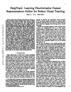
In this section experimental results obtained with the described tracking method will be proposed. Several testing sequences have been tested that proposed different difficulties as partial occlusion of non-rigid targets (PETS2006), moving camera (Scooter), and oscillating image with targets moving non uniformly (i LIDS AVSS2007). KanadeLucas-Tomasi (KLT) detector has been used to extract corner from the sequences resized to 352x288 pixels. No change detection or motion detection module is used to reduce outliers. The KLT parameters affects the tracking results in terms of sparseness or denseness of the created model and then it has to be chosen accurately. A too low number of feature will lead to a poor informative model and, on the other hand, if too many corners are added in the model the shape matching capacities are reduced. The average computational complexity of the method for a nonoptimized code is of 5 frames/sec with a 3.0 Ghz CPU with 2.0 GB of RAM. In Figure 1(a) the result on the i LIDS

(a)

(b)

Figure 1. (a) Tracking result on i LIDS AVSS sequence for frames 40, 80, 164; (b) estics,t for i LIDS AVSS sequence mated models X for frames 40, 80, 164. White points: persistence = [1,2); Green points: persistence: [2,5) ; Red points: persistence: [5,10); Cyan points: persistence > 10

Experimental results

The contribution introduced in this paper are twofold: 1) introduction of a local appearance descriptor to the tracker

AVSS sequence is presented. The sequence is oscillating due to camera movements and this leads to corners instability, i.e. from frame to frame some corners disappear and


others appear. The vehicle also slows down when it arrives close to the parked car and after it accelerates again. Despite of these issues the tracker doesn’t fail; the scale adaptation is accomplished successfully also in presence of a relevant size reduction of the target. In Figure 1(b) the estimated cs,t is represented showing with different color the model X stability with respect to previous frames, i.e. the persistence of the corners Pt . Without the usage of local information we have found that the number of element composing the model is averagely three times greater than the one here presented, 30 corners in our model, 100 corners without the patches. Moreover also the persistence tends to be higher in our model demonstrating more robust matching between model and observation elements.

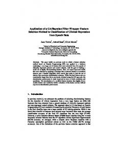
contemporary used in the ANLSE. In Figure 3 the comparison of the three methods is proposed. It can be noticed that the ANLSE (Fig. 3(a)) performs better than DNLSE (Fig. 3(b)) and NLSE (Fig. 3(c)) being able to cope with the background change due to the crossing stripes and the local luminosity change caused by the lights of the other cars. During the sequence the three (R,G,B) color combinac1 ,c2 ,c3 (see (15)) tions used to compute the weight image Ii,t before approaching to the crossing stripes were (1,1,1), (1,1,-1) and (2,-2,1). When the car move closer the stripes, the background changes lead the tracker using the obser1,1,1 vations extracted from Ii,t to fail ((20) is verified with th = 8pixels). The feature selection process is instantiated 1,1,1 and Ii,t is substituted with the color combination (0,1,2), 0,1,2 i.e. Ii,t . Though the bounding box is not properly adapted due to the persistence of two corners in the upper right are the accuracy in the stripes region is significantly better than the one of DNLSE and NLSE. In Figure 4 the trajectories

(a)

(b)

Figure 2. (a) Tracking result on i LIDS AVSS sequence for frames 40, 80, 164; (b) estics,t for PETS 2006 sequence mated models X for frames 40, 80, 164. White points: persistence = [1,2); Green points: persistence: [2,5) ; Red points: persistence: [5,10); Cyan points: persistence > 10

In Figure 2(a) the proposed method handles a partial occlusion without being distracted by the outlier corners arisen while the target is hidden by other people. The escs,t in Figure 2(b) shows that though the timated model X object deformation leads to model elements with lower persistence Pt with respect to rigid object as in Figure 1(b), cs,t represents quite well the human shape and the occluX sion don’t affect significantly the model.

4.2

Feature Adaptation Results

Different experiments have been performed on several sequence comparing the tracking method without the local descriptors (NLSE), the one using corners local appearance described in Sect. 2 (D-NLSE) and, finally the D-NLSE with the feature adaptation approach of Sect 3 (called ANLSE). In the following experiments T = 3 trackers are

(a)

(b)

(c)

Figure 3. (a) ANLSE tracking, (b) DNLSE tracking, (c) NLSE tracking. The wider bounding box is St , i.e. the searching area. of the target centroid are drawn in order to compare them to the ground truth. The accuracy improvement due to the contemporary usage of multiple trackers in the ANLSE is outlined in the first part of the trajectory where the background is simple and no light change occurs. The average tracking error with respect to the ground truth over the sequence of 85 frames are shown in Table 1. Other sequences, some of them with mobile camera, have been tested showing similar improvements with respect to DNLSE and NLSE but can

Table 1. Root Mean Square Error - RMSE in pixels for the sequence in Fig. 3 (352x288) for the ANLSE, DNLSE and NLSE method Tracking method ANLSE DNLSE NLSE

RMSE 9.3 13.1 21.8

[3]

[4]

[5]

[6]


[7]

[8]

[9]

Figure 4. Trajectories obtained from different tracking algorithm: blue) ANLSE; green) DNLSE, pink) NLSE, cyan) ground truth

[10]

[11]

not be shown in the paper for space limitations (they are attached in the supporting material).

5

[12]

Conclusion [13]

In this paper a Bayesian framework for object tracking using a corner-based shape model enriched with local appearance descriptors has been proposed. The usage of additional information aims at improving the position estimation and the model construction. An online feature adaptation strategy is integrated in this framework to automatically select the best set of features to pass to the trackers coping with different source of noise affecting them (e.g. light changes, complex background, etc.). Good performances in experimental results on difficult sequences have demonstrated the effectiveness of the algorithm.

[14]

[15]

[16]

[17]

References [18] [1] M. Asadi and C. Regazzoni. Tracking using continuous shape model learning in the presence of occlusion. EURASIP Journal on Advances in Signal Processing, 2008. [2] A. Bagdanov, A. Bimbo, F. Dini, and W. Nunziati. Improving the robustness of particle filter-based visual trackers using online parameter adaptation. In Proc. IEEE Conf.

Advanced Video and Signal Based Surveillance, pages 218– 223, Sep. 2007. R. T. Collins, Y. Liu, and M. Leordeanu. On-line selection of discriminative tracking features. IEEE Transaction on Pattern Analysis And Machine Intelligence, 27(10):1631–1643, October 2005. D. Comaniciu, V. Ramesh, and P. Meer. Kernel-based object tracking. IEEE Trans. Pattern Anal. Mach. Intell., 25(5):564–575, 2003. N. Dalal and . B. Triggs in Proc. of CVPR. Histograms of oriented gradients for human detection. In Proc. of Comp. Vision and Pattern Recognition (CVPR 2005), 2005. W. Du and J. Piater. Tracking by cluster analysis of feature points using a mixture particle filter. In Proc. of Advanced Video and Signal Surveillance (AVSS 2005), pages 165–170, Como, Italy, 2005. P. Gabriel, J. Hayet, J. Piater, and J. Verly. Object tracking using color interest points. In Proc. of Advanced Video and Signal Surveillance (AVSS 2005), pages 159–164, Como, Italy, 2005. C. G. Harris and M. J. Stephens. Combined corner and edge detector. In Proceedings of the Fourth Alvey Vision Conference, pages 147–151, 1988. M. Isard and A. Blake. Condensation – conditional density propagation for visual tracking. International Journal of Computer Vision, 29(1):5–28, 1998. L. Leung and S. Gong. Optimizing distribution-based matching by random subsampling. In Proc. of IEEE Int. Conf. on Computer Vision and Pattern Recognition, CVPR 2007, 2007. D. G. Lowe. Distinctive image features from scale-invariant keypoints. International Journal of Computer Vision, 60(2):91–110, Nov. 2004. E. Maggio, F. Smerladi, and A. Cavallaro. Adaptive multifeature tracking in a particle filtering framework. IEEE Trans. Circuits and Systems for Video Technology, 17(10):–, Oct. 2007. F. Moreno-Noguer, A. Sanfeliu, and D. Samaras. Dependent multiple cue integration for robust tracking. IEEE Trans. Pattern Analysis and Machine Intelligence, 30(4):670–685, Apr. 2008. P. P´erez, C. Hue, J. Vermaak, and M. Gangnet. Color-based probabilistic tracking. In Proc. of European Conf. on Computer Vision (ECCV 2002), 2002. C. Tomasi and T. Kanade. Detection and tracking of point features. Technical report, Carnegie Mellon University, 1991. J. Wang, X. Chen, and W. Gao. Online selecting discriminative tracking features using particle filter. In Proc. IEEE Conf. Computer Vision and Pattern Recognition, volume 2, pages 1037–1042, Jun. 2005. J. Wang and Y. Yagi. Integrating color and shape-texture features for adaptive real-time object tracking. IEEE Trans. Image Processing, 17(2):235–240, Feb. 2008. T. Woodley, B. Stenger, and R. Cipolla. Tracking using online feature selection and a local generative model. In Proc. British Machine Vision Conf., volume 2, pages 790– 799, Sep. 2007.