Online implementation of SVM based fault diagnosis strategy for PEMFC systems Zhongliang Li1,2 , Rachid Outbib2 , Stefan Giurgea1 , Daniel Hissel1 , Samir Jeme¨ı1 , S´ ebastien Rosini3 , Alain Giraud4 1 FCLAB, FR CNRS 3539, FEMTO-ST/Energy Department, UMR CNRS 6174, France. 2 LSIS, UMR CNRS 7296, Aix-Marseille University, France. 3 CEA LITEN, Grenoble, France. 4 CEA, LIST, F-91191 Gif-sur-Yvette, France.
[email protected],
[email protected],
[email protected],
[email protected],
[email protected],
[email protected],
[email protected] Keywords: PEMFC systems, Fault diagnosis, SVM, Online implementation, Robustness.
ABSTRACT This paper deals with the online diagnosis for Polymer Electrolyte Membrane Fuel Cell (PEMFC) systems. The pattern classification tool Support Vector Machine (SVM) is used to achieve fault detection and isolation (FDI). The algorithm is integrated into an embedded system of the type System in Package (SiP) and validated online in an experimental platform. Four concerned faults are diagnosed successfully online. Additionally, a procedure is proposed to improve the performance of robustness and raise the diagnosis accuracy. 1. INTRODUCTION During the last decades, fault diagnosis devoted to improve the reliability and durability performance of Polymer Electrolyte Membrane Fuel Cell (PEMFC) systems has drawn the attention of both academic and industrial communities. Through an efficient diagnosis strategy, more serious faults can be avoided thanks to an early fault alarm. With the help of diagnosis results, the downtime (repair time) can be reduced. Moreover, the precise diagnosis information can speed up the development of new technologies [1]. Several fault diagnosis strategies have been studied during the last decade. Since the first principle models of PEMFC systems are not evident to be found or estimated. The application of datadriven fault diagnosis methodologies have been drawing the attention of researchers [2]. Within the scope of data based fault diagnosis, a number of pattern classification techniques have been widely used since fault detection and isolation (FDI) can be considered as a classification problem. Thanks to the contributions from the computer science and information community, lots of mature experiences can be utilized for fault diagnosis purpose. Generally, the classification based fault diagnosis proceeds in two phases (i.e. offline phase and online phase). In the offline training phase, the historical data which distribute in different health states are firstly collected. A classifier is then trained based on the collected dataset. In the online performing phase, the real-time data are classified into the known classes with the obtained classifier. Thus, the health state of real-time data can be diagnosed. Although some classification based diagnosis strategies have been proposed for PEMFC systems [3], the online implementation results are announced rarely. Actually, for practical online applications, such as fuel cell electric vehicles, the diagnosis strategy should be integrated into an embedded system and run in real-time. Hence, the importance of online implementation cannot be overemphasized. Otherwise, the work will always stay in the step of ”academic research”. In this paper, a classification tool Support Vector Machine (SVM) is employed for FDI of PEMFC systems. The diagnosis algorithm is also integrated into a specially designed embedded system, 1
which is of the type System in Package (SiP). The embedded system is installed into a PEMFC system, and the diagnosis algorithm is verified in real-time. Besides, a procedure is proposed to improve the robustness of the diagnosis algorithm. 2. SVM BASED DIAGNOSIS ALGORITHM SVM is a classification method developed by V. Vapnik [4] and has been widely applied during the last two decades. Good generalization performance, absence of local minima and sparse representation of solution make SVM an attractive classification tool. The basic theory comes from binary classification problem. As Fig. 1 shows, there are data samples distributed in two classes, suppose we have some hyperplane which separates the points. Then, SVM looks for the optimal hyperplane with the maximum distance from the nearest training samples. A subset of training samples that lie on the margin are called support vectors. Maximum margin Support vectors
Class1 Class2
The optimal separating hyperplane
Figure 1: SVM schematic diagram
To explain the binary SVM mathematically and more specifically, take (N1 + N2 ) labeled samples z1 , z2 , . . . , zN1 +N2 from 1st and 2nd classes as training examples. gn ∈ {−1, 1} is defined as the class label of sample zn (−1 for class 1, 1 for class 2). Without going to the detailed deducing process which can be found in many materials on pattern recognition ([4] for instance), the training problem can be converted to the following quadratic problem (QP) min L(a) =
N1 +N2 NX NX 1 +N2 1 +N2 1 X an am gn gm k(zn , zm ) − an 2 n=1 m=1 n=1
(1)
subject to N1 +N2 X an gn = 0 n=1 0 ≤ an ≤ D n = 1, 2, . . . , N1 + N2
(2)
where {an |n = 1, . . . , N1 + N2 } are Lagrange multipliers, which are expressed collectively as a = [a1 , . . . , aN1 +N2 ]T ; D is a parameter which need to be initialized; k(zn , zm ) is kernel function which is introduced to solve the nonlinear problem. A representative kernel function which named Gaussian kernel is expressed as k(zn , zm ) = exp(− 2
||zn − zm ||2 ) σ
(3)
where σ is an author defined parameter. In our study, a practical approach, namely Sequential Minimal Optimization (SMO), is used solve the QP problem (1) [4]. After solving the QP problem, the Lagrange multipliers a1 , a2 , . . . , aN1 +N2 are obtained. The samples corresponding to positive Lagrange multipliers are SVs, which are denoted by z1s , z2s , . . . , zSs . S is the number of SVs. The corresponding an and gn of SV zns are denoted by asn and gns . The class label g of an arbitrary data point z can be determined by the following equation: ! S X s s s g = sign an gn k(zn , z) + b (4) n=1
where the bias b is given ! S S 1X s X s s b= gj − an gn k(zns , zjs ) S j=1 n=1
(5)
From (4), it could be observed that the determination of the class label is depended on the SVs, and the corresponding parameters {asn } and {gns }. Generally, the SVs account only a small part of the training samples. This property is central to the online applicability of SVM. The training process and the performing procedure can be synthetically summarized as Algorithm 1. Algorithm 1 Binary SVM Training: 1: Collect (N1 + N2 ) labeled sample z1 , z2 , . . . , zN1 +N2 from classes 1 and 2. gn ∈ {−1, 1}, is the class label of the sample zn . Initial D and σ. 2: Solve the quadratic problem (1) by using SMO method. s and corresponding g and a , which are denoted by {g s } and 3: Save support vectors: z1s , z2s , . . . , zS n n n {asn }. Performing: For a new sample z, its class label is determined with respect to (4).
To extend the binary classifier to multi-classification situations, there are several ways. A method named “One-Against-One” is adopted in this chapter. Actually, C(C − 1)/2 binary SVMs can be constructed based on the training data in C classes. When an arbitrary sample comes, its classification results of all the binary SVMs are firstly obtained. The final classification is obtained by voting all binary classification results. The details can be found in [5]. 3. DIAGNOSIS STRATEGY DEVELOPING PLATFORM As Fig. 2 shows, the developing platform dedicated to online implementation of the diagnosis strategy consists the following parts: PEMFC system: A 64-cell PEMFC stack, which was fabricated by the French research organization CEA specially for automotive application1 , is concerned. The nominal operating condition of the stack is summarized in Table 1. In the system, a number of physical parameters impacting or expressing stack performances can be regulated flexibly and monitored. Stack temperature, pressures and stoichiometries of hydrogen and air at inlets, relative humidity of the inlet air can be regulated. This could help causing different health states. The stack voltage and single cell voltages, as well as the above mentioned variables can all be measured with the sample time of 1 s. 1
CEA: Alternative Energies and Atomic Energy Commission
3
PEMFC system
Electronics load
Diagnosis interface Measuring & Computing unit
Figure 2: Overview of the developing platform Table 1: Nominal conditions of the stacks Parameter Value Stoichiometry H2 Stoichiometry Air Pressure at H2 inlet Pressure at Air inlet Differential of anode pressure and cathode pressure Temperature (exit of cooling circuit) Anode relative humidity Cathode relative humidity Current Voltage per cell Electrical power
1.5 2 150 kPa 150 kPa 30 kPa 65-70 ◦ C 50% 50% 90 A 0.7 V 4032 W
Electronics load: The load current can be flexibly varied through an electronic load. Measuring and computing unit: The core of the measuring and computing board is the specially-designed SiP (yellow square component shown in Fig. 2). Fig. 3 shows the structure of the SiP. The upper layer is equipped with Smartfusion on-chip system developed by Microsemi company. The device integrates a FPGA fabric, ARM Cortex-M3 Processor, and programmable analog circuitry which fulfill the A/D and D/A functions [6]. Up to 512 KB flash, 64 KB of SRAM and another two chips of 16 M memory are equipped to this SiP. With the abundant connecting ports, kinds of communications can be realized with other devices. The other two layers, which are equipped with Giant magnetoresistance (GMR) sensors, are used for measuring the voltage signals precisely. Diagnosis interface: The measurements and the calculation results obtained from the measuring and computing unit are exported to a general computer equipped with Labview software. With the help of Labview, the real-time cell voltage signals, the diagnosis results can be visualized on the screen. The real-time data can also be saved for advanced analysis.
4. ONLINE IMPLEMENTATION OF THE DIAGNOSIS STRATEGY 4.1 Offline training and algorithm integration
Knowing that classification based diagnosis belongs to supervised learning methods, the data from various classes are needed for training. To prepare the training dataset, several faults were deduced 4
MRAM EVERSPIN 16Mb (x2)
IHM FPGA JTAG SPI+CAN Smartfusion: communications A2F500 Other functions
GMR channels
E/S Annexes
FPGA Smartfusion
Memory
GMRs
Amplifiers
GMRs
Amplifiers
Analog signals transfer
Figure 3: SiP designed for PEMFC system diagnosis [7]
deliberately. Table 2 summarizes the operations in the experiment of training data preparation. In this study, the individual cell voltages are considered as the variables for diagnosis. From our previous study, individual cell voltages show different magnitudes and distributions in different health states. This feature is utilized for FDI. Constrained by the measuring capability of the 1st version SiP. The voltages of 14 cells which located near to one side of the stack can be measured and used as the variables for diagnosis. The evolutions of individual cell voltages of training data are shown in Fig. 4(a). Table 2: Experimental procedure for the preparation of training dataset Starting time
Ending time
Operation
Health state
0 880 1676 2619 3500 4893 6289 7519 8288
879 1675 2618 3499 4892 6288 7518 8287 8955
Nominal condition Pressure at 1.3 bar at each side Back to nominal condition Pressure at 1.7 bar at each side Back to nominal condition Lower relative humidity Back to nominal condition St. Air 1.5 Back to nominal condition
Normal state (Nl) Low pressure fault (F1) Normal state (Nl) High pressure fault (F2) Normal state (Nl) Drying fault (F3) Normal state (Nl) Low air stoichiometry fault (F4) Normal state (Nl)
Table 3: Confusion matrix for training data Nl
Actual classes
Nl F1 F2 F3 F4
4762 406 300 157 239
Diagnosed classes F1 F2 F3 29 373 0 11 82
25 0 800 0 0
68 0 0 1228 0
F4 11 17 0 0 448
With the training dataset, the SVM classifier is trained. Classifying the training data with the trained SVM, the diagnosis accuracy rate is 84.98%. More detailed diagnosis results can be summarized as a confusion matrix shown quantitatively in Table 3 and visually in Fig. 4(b). It could be observed that the false alarm rate, i.e. the rate of the samples in normal state are wrongly 5
Actual class Diagnosis class F4
Class
F3
F2
F1
N 0
1000
2000
3000
4000
5000
6000
7000
8000
9000
Time [s]
(a) Evolutions of cell voltages: training data
(b) Diagnsois results: training data
Figure 4: Training data and diagnosis results
diagnosed into the fault classes, is relatively low. The diagnosis accuracy for the data in F3 is high, while a considerable part of data in classes F1, F2, and F4 are wrongly classified into the normal class. The trained SVM classifier was coded into the memory of SiP. When the diagnosis algorithm was carried out using the training dataset respectively in MATLAB environment and the SiP, the accordant results could be obtained. Besides, the diagnosis algorithm could be calculated within a sampling cycle (i.e. 1s) using the SiP. That is to say the diagnosis algorithm is successfully integrated into the embedded system. 4.2 Online validation
To realize online validation, the embedded system was tested online with the real-time data during another experiment. The operations of this experiment are summarized in Table 4, and the measured cell voltages (i.e. the variables for diagnosis) are plotted in Fig. 5(a). The diagnosis accuracy of the online implementation is 85.93%. Similarly, the online diagnosis results were recorded and summarized visually in Fig. 5(b) and quantitatively in Table 5. A similar observation as the case for training could be obtained when the confusion matrix (i.e. Table 5(b)) of test data is analyzed. Table 4: Experimental procedure for online validation Starting time
Ending time
Operation
Health state
0 3661 4544 5375 6542 9842 8910 8129 11910
3660 4543 5374 6541 8128 11909 9841 8909 12459
Nominal condition Pressure at 1.3 bar at each side Back to nominal condition Pressure at 1.7 bar at each side Back to nominal condition St. Air 1.5 Back to nominal condition Lower relative humidity Back to nominal condition
Normal state (Nl) Low pressure fault (F1) Normal state (Nl) High pressure fault (F2) Normal state (Nl) Low air stoichiometry fault (F4) Normal state (Nl) Drying fault (F3) Normal state (Nl)
6
Actual class Diagnosis class F4
Class
F3
F2
F1
N 0
2000
4000
6000
8000
10000
12000
14000
Time [s]
(a) Evolutions of cell voltages: test data
(b) Diagnosis results: test data
Figure 5: Test data and diagnosis results 4.3 Improvement of the robustness and accuracy
When the faults F1, F2, and F4 are concerned, it can be observed from the Fig. 5(b) that the diagnosis results vibrate between the corresponding fault and normal classes. The performance of robustness is not satisfying. Here we propose to use a lagged results to improve the robustness and accuracy of the diagnosis results. Specifically, at time k, the diagnosis results of last Nlag are taken into account (i.e. from k − Nlag + 1 to k). Concerning these Nlag data, if fault degree (i.e. the rate of one fault diagnosed) is above the pre-defined threshold, the fault occurs at time k. Here we set Nlag = 100 and threshold as 0.4. The fault degrees of the concerned four faults are shown in Fig. 6(a). The diagnosis results are shown in Fig. 6(b) and Table 6. Comparing Fig. 6(b) to Fig. 5(b), more consistent and robust results can be obtained when fault degree is used as the indicator of the faults. Considering diagnosis accuracy, the global diagnosis accuracy is 93.54% which is significantly improved. Notice that sensitivity and robustness are two conflicting factors, the performance of sensitivity is certainly alleviated when the procedure is employed. Table 5: Confusion matrix for test data Diagnosed classes Nl F1 F2 F3
Actual classes
Nl F1 F2 F3 F4
7302 446 477 142 363
31 432 0 28 14
220 0 690 5 14
0 1 0 1880 0
F4 10 4 0 8 390
5. CONCLUSION In this paper, classification method SVM is used to realized fault diagnosis for PEMFC systems. The algorithm was successfully integrated into a specially designed embedded system. The integrated system was installed into a PEMFC system and tested online. Four faults can be detected and isolated. The robustness and diagnosis accuracy performances are improved by introducing the concept of fault degree. The total diagnosis accuracy can arrive at 93.54%.
7
F1 F2 F3 F4
1 0.9
Actual class Diagnosis class F4
0.8 F3
0.6
Class
Fault degree
0.7
0.5
F2
Threshold
0.4 0.3
F1
0.2 0.1 0
N 0
2000
4000
6000
8000
10000
12000
14000
0
2000
4000
Time [s]
6000
8000
10000
12000
14000
Time [s]
(a) Fault degrees of 4 faults
(b) Diagnosis results: test data
Figure 6: Improved diagnosis results Table 6: Confusion matrix for test data: improved results Nl
Actual classes
Nl F1 F2 F3 F4
7413 215 88 202 150
Diagnosed classes F1 F2 F3
F4
0 668 0 0 0
40 0 0 0 631
62 0 1079 0 0
48 0 0 1861 0
ACKNOWLEDGMENT The work is a contribution to the ANR DIAPASON2 project. The authors would like to thank the ANR for funding the project. REFERENCE [1] Z. Li, Data-driven fault diagnosis for PEMFC systems. PhD thesis, Aix-Marseille University, 9 2014. [2] Z. Zheng, R. Petrone, M. P´era, D. Hissel, M. Becherif, C. Pianese, N. Yousfi Steiner, and M. Sorrentino, “A review on non-model based diagnosis methodologies for PEM fuel cell stacks and systems,” International Journal of Hydrogen Energy, vol. 38, pp. 8914–8926, July 2013. [3] Z. Li, R. Outbib, D. Hissel, and S. Giurgea, “Data-driven diagnosis of PEM fuel cell: A comparative study,” Control Engineering Practice, vol. 28, pp. 1–12, July 2014. [4] J. C. Platt, “Sequential Minimal Optimization : A Fast Algorithm for Training Support Vector Machines,” Technical Report MSR-TR-98-14, Microsoft Research, pp. 1–21, 1998. [5] C.-W. Hsu and C.-J. Lin, “A comparison of methods for multiclass support vector machines,” Neural Networks, IEEE Transactions on, vol. 13, no. 2, pp. 415–425, 2002. [6] “Website: Smartfusion introduction.” [7] A. GIRAUD, “Embedded smart sensors for measurement and diagnosis of measurement and diagnosis of multicells pemfc.” Report - project DIAPASON, June 2012. 8