IEEE TRANSACTIONS ON SYSTEMS, MAN, AND CYBERNETICS—PART B: CYBERNETICS, VOL. 34, NO. 4, AUGUST 2004
1811
Online Monitoring by Dynamically Refining Imprecise Models Bernhard Rinner, Senior Member, IEEE, and Ulrich Weiss
Abstract—Model-based monitoring determines faults in a supervised system by comparing the available system’s measurements with a priori information represented by the system’s mathematical model. Especially in technical environments, a monitoring system must be able to reason with incomplete knowledge about the supervised system, to process noisy and erroneous observations and to react within a limited time. We present MOSES, a model-based monitoring system which is based on imprecise models where the structure is known and the parameters may be imprecisely specified by numerical intervals. As a consequence, only bounds on the trajectories can be derived with imprecise models. These bounds are computed using traditional numerical integration techniques starting from individual points on the external surface of the model’s uncertainty space. When new measurements from the supervised system become available, MOSES checks the consistency of this new information with the model’s prediction and refutes inconsistent parts from the uncertainty space of the model. A fault in the supervised system is detected when the complete model’s uncertainty space has been refuted. MOSES bridges and extends methodologies from the FDI and DX communities by refining the model’s uncertainty space conservatively through refutation, by applying standard numerical techniques for deriving the trajectories of imprecise models and by exploiting the measurements as soon as possible for online monitoring. The performance of MOSES is evaluated based on examples and by online monitoring a complex heating system. Index Terms—Imprecise models, model-based monitoring, parameter estimation, uncertainty space partitioning.
I. INTRODUCTION
T
HE PRIMARY objective of monitoring is to detect abnormal behaviors of a supervised system as soon as possible to avoid shutdown or damage. Due to the increased complexity of many supervised systems, monitoring is becoming more and more important. Physical systems especially, such as robots, production lines, or anti-lock brakes provide a vast number of challenges for a monitoring system. In such an environment, the monitoring system must be able to reason with incomplete knowledge about the supervised system, to process noisy and erroneous observations, and to react within predefined time windows.
Manuscript received July 14, 2002; revised September 5, 2003. This work was supported in part by the Austrian Science Fund under Grant Number P14233-INF. This paper was intended for the Special Section on Diagnosis of Complex Systems: Bridging the Methodologies of the FDI and DX Communities which is to appear in 2004. This paper was recommended by Associate Editor L. Trave-Massuyes. The authors are with the Institute for Technical Informatics, Graz University of Technology, A-8010 Graz, Austria (e-mail:
[email protected];
[email protected]). Digital Object Identifier 10.1109/TSMCB.2004.828592
A particularly important and widely-applied approach is model-based monitoring [1] which can be defined as the determination of faults in a supervised system from the comparison of available system’s measurements with a priori information represented by the system’s mathematical model [2]. A discrepancy between the derived system’s behavior and the observed behavior indicates a fault in the supervised system. Model-based monitoring techniques have been investigated and developed within the diagnosis (DX) [3]–[5] and the Fault Detection and Isolation (FDI) [6]–[8] communities over the last few years. Model-based monitoring makes use of mathematical models of the supervised system. However, a perfectly accurate and complete model of a physical system is almost never available. Usually, the parameters of the system may vary with time in an uncertain manner, and the characteristics of the disturbances and noise are unknown so that they cannot be modeled accurately. Hence, there is a mismatch between the physical system and its mathematical model even if there are no faults present. For model-based monitoring, it is therefore important how to express and reason with incomplete knowledge. Traditional FDI methods for model-based monitoring are essentially based on numerical methods such as state estimation and parameter estimation [9]–[11]. The general structure of such a FDI system consists typically of two stages. First, fault indicating signals, i.e., residuals, are generated using available input and output data of the supervised system. Second, the residuals are examined for the likelihood of faults, and a decision rule is then applied to determine if any faults have occurred. Incomplete knowledge is often represented by parameterized differential equations. We present an alternative approach to model-based monitoring of physical systems (called MOSES, for MOnitoring using uncertainty Space partitioning for physical systEmS) that combines and extends techniques from DX and FDI. Our approach [12]–[14] is based on imprecise models1 where the structure of the models is known and the parameters may be imprecisely given as numerical intervals. These parameter intervals span the uncertainty space of the model. Only bounds on the trajectory, i.e., envelopes, can be derived from an imprecise model based on intervals. However, it is in principle not possible to decide whether a supervised system is fault-free by using imprecise models, since the output of a faulty system can lie anywhere, i.e., inside or outside the envelopes. In order to reduce missed alarms 1Remember the difference between precision and accuracy. Precision refers to the degree of specified detail which can be observed or predicted from a model, while accuracy refers to the truthfulness, or correctness, of the specified or predicted data.
1083-4419/04$20.00 © 2004 IEEE
1812
IEEE TRANSACTIONS ON SYSTEMS, MAN, AND CYBERNETICS—PART B: CYBERNETICS, VOL. 34, NO. 4, AUGUST 2004
and reduce the fault recognition times it is, therefore, important to keep the envelopes small. MOSES achieves small envelopes by applying numerical integration techniques for solving imprecise models and by checking the consistency of the observed data with the model’s prediction whenever new measurements are available. It removes then inconsistent parts from the uncertainty space of the model. Our approach bridges and extends methodologies from the FDI and the DX communities in the following way. 1) Modeling the incomplete knowledge about the supervised system is based on differential equations which are augmented by numerical intervals of parameters. In general, reasoning with intervals is complex and tedious. However, by focusing only on individual points on the surface of the model’s uncertainty space, we can use standard numerical methods, i.e., Runge–Kutta integration, for deriving the envelopes. 2) Measurements and prediction are checked for consistency by exploiting qualitative information from the residuals. Discrepancies are only reported when there is no overlap between the measurements and the predicted envelopes. 3) By refuting parts of the uncertainty space that are inconsistent, MOSES also performs model refinement during monitoring. This technique originates from semi-quantitative system identification [15], [16] and is related to interval analysis [17], [18]. We have extended and applied this technique to online monitoring. By exploiting measurements as soon as possible for online monitoring by refining the uncertainty space conservatively through refutation and by applying standard numerical techniques for deriving the trajectories of imprecise models, our approach combines and complements techniques from FDI and DX and helps make them more widely and robustly available. The remainder of this paper is organized as follows. Section II presents the basic monitoring approach of MOSES, i.e., it describes the imprecise modeling, the partitioning of the model’s uncertainty space and the checking for consistency with the measurements. Section III extends the basic monitoring approach. The problem of nonmonotonicity of state variables is discussed, and a check for monotonicity is introduced. We also discuss the limitations of the basic approach for oscillating systems and how this problem is solved by intersecting the measurements with the predicted envelopes. Section IV presents experimental results of our implemented monitoring system. Section V discusses related work and Section VI concludes this paper with a discussion and an outlook for future work. II. MONITORING BY REFUTING SUBSPACE MODELS A. Overview Monitoring methods based on imprecise models can reason with incomplete knowledge in the model as well as with noisy measurements. A main drawback of the standard interval approach, however, is that the envelopes may diverge very rapidly which delays or even inhibits a fault recognition. We have revised this interval approach to model-based monitoring with the
primary goal to keep the resulting envelopes as small as possible. In our approach, we exploit the measurements from the supervised system as soon as possible to refine the uncertainty in the model and the derived envelopes. The key step in our approach is to partition the uncertainty space of the model into several subspaces. The trajectories derived from each subspace are then checked for consistency with the measurements. Each inconsistent subspace is refuted and excluded from further investigations. Partitioning and consistency checking are continued resulting in a smaller uncertainty space of the model and smaller envelopes. When all subspaces are refuted, a discrepancy between the model prediction and the observation has been recognized and a fault has been detected. Like uncertain parameters, measurement noise can also be represented by numerical intervals in MOSES. B. Imprecise Modeling and Subspace Partitioning In general, a physical system can be modeled as a differential equation of order (1) is the state vector at time is the input vector at where time is the parameter vector at time is the output vector at time , and and are vector functions. In a precise is a vector of real numbers. However, in a model model, can be replaced by a vector of with uncertain parameters, intervals where is the number of uncertain parameters.2 A model with uncertain parameters, i.e., an imprecise model, can therefore be described as (2) Equation (2) is the starting point of our approach. It defines an imprecise model of the supervised system with uncertain parameters. This model has a -dimensional uncertainty space. A partition is defined as (3) . Thus, a partition divides the uncertainty space into with smaller regions. A model based on a partition of the uncertainty space is referred to as a subspace model which has obviously less imprecision than the unpartitioned model. In order to apply subspace models to monitoring, a complete partitioning into partitions must satisfy the following condition: where . Thus, the union of all subspace models covers the complete (initial) uncertainty space of the imprecise model. Note that the individual partitions may overlap. The system equation of a subspace model is formally defined as:
(4) 2In our approach we assume that the parameters do not vary over time and are not necessarily independent.
RINNER AND WEISS: ONLINE MONITORING BY DYNAMICALLY REFINING IMPRECISE MODELS
1813
To apply imprecise models in MOSES, we must compute their trajectories. A simple but intractable method to derive the trajectories is to repeat a numerical integration starting from any point within the uncertainty space.3 If we assume monotonicity and with regard to the parameters over the range of of the intervals, it is sufficient to focus only on a few points of the uncertainty space. C. Consistency Checking With the monotonicity assumption, the (imprecise) state of a subspace model can be represented by the (precise) state at extremal points, i.e., corner points, of a subspace. The corner points of a subspace are defined as all combinations of upper and lower bounds of a partition and can be represented as with . Thus, an uncertainty set space of dimension results in corner points. The states at the corner points can be represented as set
(5) is a numerical parameter vector from the subspace where and at corner of this subspace. are are output vectors both with nustate vectors, and also merical values.4 This representation of an uncertain state is directly exploited by our consistency check for a given subspace . First, a residual vector is calculated for each state at a corner point using the measurements at time , i.e., . represents the measured output values of the supervised system. has the same dimension as and . Then, the minimum and maximum values of the residual are determined for each measured variable over all corner points as (6) (7) with , and . Finally, the subspace model is checked for consistency by simply comparing the signs of and . The subspace model is consistent with the measurements, iff (8) holds for all elements
.
3Note that for deriving the trajectories of imprecise models, it is also sufficient
to focus on points belonging to the external surface of the uncertainty space [19]. However, the number of trajectories to be computed is still infinite, even if it is of a lower order. 4Note that our basic approach requires a precise initial state x(t ) for the computation of the state at time t using standard numerical methods such as Runge-Kutta integration. As we see in the next section and also in [14], MOSES can be used with imprecise initial states. In this case, the imprecise initial state is represented by additional uncertain parameters.
Fig. 1. Consistency check with one uncertain parameter p and three subspaces , and q~ . The residuals at the corner points of subspace q~ are both negative, therefore, the model with the subspace q~ is inconsistent with the measurement. In subspace q~ , the residuals at the corner points have different signs. Thus, q~ is consistent. For the parameter range of subspace q~ the monotonicity assumption is violated. In this case, checking the residuals’ signs at the corner points is not feasible. q ~ ; q~
Informally, (8) checks whether the zero vector lies within the “residual subspace” (see Fig. 1). If this equation is violated, the is refuted. This simple consistency check subspace model also holds if all elements of are not included in the measurements. In this case, a comparison with the missing elements is simply ignored. Since this technique is based on the calculation of a precise state (at corner points), we can use standard numerical methods for computing the solution of differential equations. Subspace models are only refuted when they are inconsistent with the measurements. D. Dynamic Partitioning At the beginning of a monitoring process the imprecise model of the supervised system is partitioned into several subspace models. During monitoring, a large number of these subspace models may be detected as inconsistent; only a few subspace models remain consistent. To increase the fault detection performance of MOSES, the uncertainty space of the consistent subspace models can be partitioned dynamically during monitoring. At any time a consistent subspace can be partitioned into smaller subspaces as long as (3) holds. This dynamic partitioning results in smaller subspace models that potentially describe the supervised system more precisely. There is clearly a trade-off between the number of (active) subspace models and the computational load in MOSES. Dynamic partitioning allows to adjust online the computational load as well as the degree of uncertainty of individual subspaces. Dynamic partitioning also reduces the problem of accumulation uncertainty of imprecise models. In general, the predicted uncertainty of imprecise models increases over time resulting in diverging envelopes. An additional source of uncertainty in physical systems is measurement noise. In MOSES, noise can be simply handled as additional uncertain parameters, i.e., the measurements are superimposed by a fixed (noise) interval. The residual is then computed using this interval. Note that uncertain parameters representing measurement noise may not be divided during dynamic partitioning.
1814
IEEE TRANSACTIONS ON SYSTEMS, MAN, AND CYBERNETICS—PART B: CYBERNETICS, VOL. 34, NO. 4, AUGUST 2004
III. EXTENSIONS When the monotonicity of the state variables is given, the envelopes computed by numerical integration starting from the extremal points are sound and complete [19]. Such envelopes are also referred to as “exact” envelopes [20] and represent the optimal output for an interval simulator. When the monotonicity is not given, MOSES computes underbounded envelopes which lie within the exact ones. However, underbounded envelopes can not be used to check the consistency with the measurements and to refute subspace models. In this section, we analyze the monotonicity assumption and extend the basic monitoring approach of MOSES in the following way. First, a check for monotonicity is included and subspace models are checked (and potentially refuted) only when the monotonicity has been positively checked. Second, MOSES is able to introduce a new initial state each time new measurements are available. By these extensions MOSES is then able to: 1) monitor systems even if its imprecise model violates the monotonicity assumption for limited periods of time and 2) reduce the uncertainty by intersecting measurements with predicted envelopes.
Fig. 2. Illustrative example for checking the monotonicity of a system with one state variable x and one parameter p. To check the subspace model for monotonicity, the gradients of the state values with regard to the parameters are calculated at the corner points. In this example, the subspace q~ is monotonic and the subspace q~ violates the monotonicity check.
model may become monotonic again, and the consistency check can then be applied again. The monotonicity of the state values for an individual subspace is checked by comparing the sign of the gradients of the state values with regard to the parameters (cp. Fig. 2) at the corner points of each subspace. We start the computation of the matrix for the monotonicity by defining a partial derivatives of the state values’ derivatives, i.e., the matrix elements are given as
A. Nonmonotonicity of State Values In general, the monotonicity of the state values with regard to the parameters cannot be guaranteed by the monotonicity of the system equations and . For example, the monotonicity may not be given when one of the following conditions is violated: 1) the system input does not change; 2) the initial values of a subspace model are independent of the parameters; and 3) all eigenvalues of the system model are real valued. The first condition is especially relevant for controlled processes or hybrid system models [21] which can change the system’s input either continuously or discretely. The second condition is a simple consequence of the integration of the . If the given differential equation: initial states are different at some corner points in the need not be monotonic subspace model, the state values (even if is monotonic) with regard to the parameter. However, this potential nonmonotonic behavior appears only for a limited period of time. The third condition corresponds to nonoscillating systems because in an oscillating system monotonicity cannot be guaranteed for an arbitrary time. These are very restrictive conditions and limit the applicability of our basic monitoring approach. To overcome these limitations, we have extended our basic approach.
(9) where is the time, is the state vector, and is the parameter vector with its elements . For determing the monotonicity of the state values with regard to the parameters, we need the matrix with the elements (10) Similar to [19], the matrix
(11) where
(the empty matrix), and matrix 5
is defined as (12)
The elements represent the trend of the state value with regard to the parameter . This is exploited by our monotonicity check: The state values of a subspace model are monotonic iff
B. Checking for Monotonicity As discussed above, there are several conditions which may result in a nonmonotonicity of the state values with regard to the parameters (for a limited period of time). This nonmonotonicity may lead, in turn, to underbounded envelopes and an incorrect consistency check. Thus, to maintain a correct (and conservative) monitoring technique, we must precede MOSES’ consistency check by a check for monotonicity.If the state values of a subspace model are detected as nonmonotonic, the consistency check is simply bypassed. This subspace can be neither accepted nor refuted at that time. After some time the subspace
is computed by
(13) holds for all state values and all directions of . represents the the uncertainty space at the corner point with the minimum value of (cp. (6)). represents the value residual of subspace of at the corner point with the maximum residual [cp. (7)]. The computation of this monotonicity check implies a numerical solution of the differential equation (11). 5For linear systems matrix, tion matrix.
A is constant and corresponds to the state transi-
RINNER AND WEISS: ONLINE MONITORING BY DYNAMICALLY REFINING IMPRECISE MODELS
1815
Fig. 3. The monotonicity check is demonstrated on the simple example of an oscillating system. The monotonicity of x (t; p) is checked at time t by comparing the signs of the state derivatives at the corner points. Three cases can be distinguished: (a) the state variable is correctly detected as monotonic (M1); (b) the state variable is correctly detected as nonmonotonic (M2); and (c) after t = 2, the state variable is nonmonotonic but may be wrongly detected as monotonic (M3).
C. Oscillating Systems In general, the trajectories of oscillating systems have different periods due to the interval ranges of the uncertain parameters. The state values are, therefore, only monotonic as long as the deviation between the maximum and minimum frequency is small. Clearly, this deviation increases with time. We demonstrate the effect of diverging frequencies on a small example. Consider the following system with two state variables and a single parameter
(14) With the initial state vector system is given as
, the solution of this
(15) (16) The derivative of the state variables with regard to the parameter is (17) (18) In this example, we only consider the first state variable (15). For a given parameter we can distinguish between three regions concerning the monotonicity of
To solve this problem of oscillating systems, we have taken a closer look at the cause of the nonmonotonicity. In general, the solution of a linear system has the following form: (20) where can be complex and are monotonic with regard are the imaginary parts of the eigenvalues, to and . , and is the time from the initial state. The exponential term can also be expressed as a combination of sinus and cosinus functions which are of course nonmonotonic: . is monotonic, if Considering only the real part, . As long as this inequality is satisfied, monotonicity of the state values is guaranteed. This can be achieved small or 2) by keeping by two approaches: 1) by keeping the integration time small. is a property Concerning the first approach, note that of the supervised system and, therefore, cannot be influenced by our algorithm. However, the system states have to be monotonic only within an individual subspace model. The states in the subspace model are monotonic if (21) holds, where for all eigenvalues of the are the corner points of the subsystem and space. The monotonicity check, however, is able to detect the monotonicity, only as long as the deviation between maximum and minimum frequencies of the state does not exceed a complete cycle within the subspace [see Fig. 3(c)]. Thus, the monotonicity check is only valid if (22)
(19) These three cases concerning the monotonicity of are depicted in Fig. 3. In general, the dynamics of the system cause the states to be nonmonotonic with regard to the parameters after a certain time. After that time it is, therefore, not possible to refute any subspace; monitoring would become infeasible with our basic approach.
holds. Note that (21) and (22) correspond to the border between the regions and as well as and of (19), respectively. Concerning the second approach, since time increases steadily from an initial state, all subspace models will eventually become nonmonotonic [cp. (22)] and, thus, our monitoring algorithm would be useless for oscillating systems without modification. The measurements from the supervised system, however, do provide some information about the time, and we
1816
IEEE TRANSACTIONS ON SYSTEMS, MAN, AND CYBERNETICS—PART B: CYBERNETICS, VOL. 34, NO. 4, AUGUST 2004
can exploit this information so that a new initial state can be introduced at each sampling point. The (integration) time is then limited by the sampling period. Introducing new initial states by exploiting the measurements from the supervised system is discussed in the following section in more detail. D. Intersecting the Measurements With the Trajectories The key step of this modification is to introduce an initial state each time new measurements are available. If the sampling period is small with regard to the dynamics of the supervised system—which is normally the case —(22) is satisfied and the monotonicity information is guaranteed. In order to introduce a new initial state, the measurements must be intersected with the computed trajectories (Fig. 4). Since measurements as well as trajectories include uncertainty due to noise and uncertain parameters, the intersection also includes uncertainty. This results in an (imprecise) initial state space for our monitoring algorithm. Measurement noise is represented by superimposing a predefined interval over all measured variables resulting in a measurement space. Clearly, an initial state space introduces additional uncertainty to our algorithm. When starting from an initial state space, our monitoring algorithm computes an individual trajectory of each extremal point of the initial state space. This results in several uncertain state spaces which can be bound by a single uncertainty space, i.e., the computed trajectory space. (cp. rectangles C and B in Fig. 4). The computed trajectory space is larger than the sum of the individual uncertain state spaces. We can distinguish four different cases for the generation of the new initial state space at time in our modified algorithm. These cases are referred to as initial state cases which have different effects on the accumulation of uncertainty and the duration of the integration time. Case 1) Take the measurement space as initial state space (rectangle E in Fig. 4). In this case, the measurement provides significant new information about the uncertainty of the state space. By using the measurement space as new initial state space, the accumulating uncertainty effect is not relevant. The integration time is limited by the sampling period. Case 2) Take the computed trajectory space as initial state space (rectangle B in Fig. 4). In this case, the measurement does not provide any new information and, thus, the computed trajectory space must be used as new initial state space. The accumulating uncertainty effect is relevant; the integration time is limited by the sampling period. Case 3) Take the intersection as initial state space (rectangle F in Fig. 4). In this case, the intersection between trajectory and measurement space is used as new initial state space which is the smallest space of the four cases. No accumulating uncertainty effect appears, and the integration time is limited by the sampling period. Case 4) Continue with the corner points (rectangles C in Fig. 4). When measurements do not provide any information or are not available at all, we continue the
Fig. 4. Intersection of trajectories and measurements in the state space. The initial state space at time t 1 is represented by rectangle A. Due to parameter uncertainty, this initial state space results in several uncertainty spaces at time t (rectangles C) which can be bounded by a single uncertainty space (rectangle B). Point D represents the measurement at time t; measurement noise is accounted by rectangle E. Rectangle F is the result of the intersection and may serve as new initial state space at time t.
0
computation of the trajectories with the corner points of the uncertainty space. No new initial state space is introduced. Thus, we achieve a medium level for the accumulating uncertainty (better than case 2); the integration time increases. The four initial state cases are depicted in Fig. 4. Note that for determining the initial space of each state variable any of the cases 1 to 3 can be chosen. Obviously, case 4 can only be applied jointly for all state variables. The remaining open question is now what initial state case should we choose. Since monotonicity may not be given for all state variables and not all state variables may be measured, several cases have to be considered. In principle, the new initial state space at time is determined by the following rules. 1) If a measurement for state variable is available at and is monotonic, then the intersection between trajectory and measurement is taken as new initial state space for (case 3). If the intersection is empty, the subspace model is refuted. 2) If a measurement for state variable is available at and is not monotonic, we cannot decide the consistency between trajectory and measurement. In order to keep the integration time small, the measurement space is used as new initial state space for (case 1). 3) If a measurement for state variable is not available at and is monotonic, then the computed trajectory space is used as new initial state space for (case 2). 4) If a measurement for state variable is not available at and is not monotonic, then we have to continue with the corner points of the uncertainty space (case 4). The algorithm for selecting the new initial state space is presented in Fig. 5. This algorithm replaces the simple consistency check of the basic algorithm in MOSES. It determines the new initial state space in three consecutive steps. First, it checks all state variables where measurements are available and determines whether the intersection or the measurement are used as new state space for that variable. Second, it checks the re-
RINNER AND WEISS: ONLINE MONITORING BY DYNAMICALLY REFINING IMPRECISE MODELS
1817
Fig. 5. Pseudo code for the consistency check with initial state space selection.
Fig. 6. Initial state cases in a two-dimensional state space. Depending on the position of the measurement and trajectory space the new initial state space can be distinguished.
maining state variables, and finally the overall initial state space is generated. Fig. 6 depicts some examples of the selection of the new initial state space based on a two-dimensional state space. Fig. 6(a) depicts the case where measurements of both state variables are available and the measurement space is completely overlapped by the computed trajectories. Thus, the measurement space is taken as the new initial state space. In Fig. 6(b), the measurement space is only overlapped by the computed trajectory space is monotonic can the subspace model be in . Only when is not monotonic, then this measurement may be refuted. If consistent. Figs. 6(c) and (d) show examples where no measureare available. The initial state space for this variments for able can only be bounded by the computed trajectories, if is monotonic. For the measured variable , the monotonicity decides whether the measurement space or the intersection is taken. As mentioned above measurements for all state variables are not always available. In general, the measurement gives us information about the output vector , and not the state vector itself. For linear systems, the differential equation model in (1) , with can be transformed into , and . We appropriate dimensions for the matrixes and to calculate the state vector: can use the matrixes . If is not regular, i.e., , not
all state values can be derived from the measurements. In this case, we can remove certain columns from as well as the corresponding state values. The reduced matrix will then become regular and the values for certain variables can be derived. IV. EXPERIMENTAL RESULTS The monitoring system MOSES has been completely implemented on a standard PC running Linux. The software has been implemented in C/C++. The performance of MOSES is evaluated using both a simulated as well as a “real” supervised system. The evaluation is performed in both offline and online operation. We demonstrate the performance of MOSES in three different areas. First, we compare the basic monitoring algorithm with the modified algorithm using an oscillating system. Second, we demonstrate the fault detection performance of MOSES in a realworld example. Finally, we demonstrate how MOSES is able to refine uncertain parameters during monitoring. A. Comparison Between the Basic and the Modified Algorithm This comparison is based on a simulated supervised system. Consider again the linear system
(23)
1818
IEEE TRANSACTIONS ON SYSTEMS, MAN, AND CYBERNETICS—PART B: CYBERNETICS, VOL. 34, NO. 4, AUGUST 2004
Fig. 7. Oscillating system (23) monitored with the basic MOSES approach. x (a) and x (b) are plotted each with the envelopes (solid line), and the measurements including a noise interval (vertical lines). The monotonicity regions are marked at the bottom of the diagrams. The monitoring process terminates at t = 4 because MOSES wrongly detects an inconsistency between measurements and trajectories.
with two state variables and and a single uncertain parameter . The initial state values are given as and . The parameter . In this experiment, (23) is interval is given as . The values of both state variables are simulated with superimposed by random noise within to generate the “measurements” for MOSES. The sampling period is given as 0.1 s. These measurements are clearly consistent with the computed trajectories of the imprecise model. We first monitor the oscillating system using the basic algorithm, i.e., trajectories and measurements are not intersected and no new initial states are introduced. Monitoring without inter, because MOSES wrongly section (see Fig. 7) terminates at detects an inconsistency between measurement and trajectory. This error is caused because (22) is violated, and our monotonicity check assumes monotonic states. In MOSES, the monotonicity check is applied at each sampling time. The monotonicity regions M1 to M3 corresponding to (19) are also depicted in Fig. 7. Note that an inconsistency between trajectory and measurement can only be genuinely detected by MOSES in region M1. In contrast, Fig. 8 depicts the monitoring process of MOSES using the modified algorithm, i.e., an intersection between measurement and trajectory is performed and new initial states are introduced. In this case, MOSES is able to accept all measurements until the simulation ends at . Note that the states remain almost always monotonic, i.e., within monotonicity re-
Fig. 8. Oscillating system (23), monitored with the extended MOSES approach. The monitoring process genuinely accepts all measurements and ends at t = 11.
gion M1. This is because the integration time is kept small by introducing new initial state spaces at every sampling period. B. Fault-Detection Performance We demonstrate the performance of our monitoring algorithm on a “real” physical system which is comprised of three heating/cooling components mounted on a thermal conductive plate. A process control computer (B&R 2003) controls the three heating/cooling components. The measured samples as well as the control actions issued are transferred to MOSES via a RS 232 interface. Our model, which includes the three components with heating elements, is given as
(24) where is the temperature of the three components, is the mass of the components, is the heat flow into the components, is the thermal conductivity between the component and the environment, is the thermal conductivity between the comis the temperature of the environment. ponents and , and We can reduce the complexity of this model by exploiting the symmetric construction of the heating system resulting in a total of five uncertain parameters. , the input The state vector is given as , and the output vector as vector as
RINNER AND WEISS: ONLINE MONITORING BY DYNAMICALLY REFINING IMPRECISE MODELS
(a)
1819
(b)
Fig. 9. Scenario of (a) an intermittent fault and (b) fault detection by observing temperature sensor T3. The sensor readings of all four temperature sensors as well as the induced fault are plotted in the left graph. The derived trajectories and the sensor reading for temperature sensor T3 are plotted in the right graph. TABLE I TIME REQUIRED TO DETECT THE INTERMITTENT FAULT USING MOSES
. The noise interval of the temperature sensors is set to 0.3. W We have measured the input values with and W (the heating element is either turned off or turned on).6 After an initial refinement step of MOSES, we get the parameter intervals as . This refinement step is performed in a single continuous behavior segment [12]. We demonstrate the fault detection performance using an intermittent fault scenario in component 3 of the heating system the heating element of component 2 is [Fig. 9(a)]. At switched on; all other actuators remain turned off. Starting at s, the heating element of component 3 is switched on and off several times. Fig. 9(b) depicts the situation of detecting this fault scenario by observing only the temperature sensor of , the sensor value exceeds the trajeccomponent 3. At tory derived from the imprecise model. Note that the envelopes are kept quite small all the time. Table I presents the time required by our monitoring system for detecting the intermittent fault in the heating system. This table summarizes the results from experiments where the uncertainty space of the model and the number of observed variables have been varied. Model #1 has the largest uncertainty space and model #4 has the smallest uncertainty space. The parameter intervals of these models are presented in Table III. Note that observing only T1 is not sufficient in order to detect the fault within the observation period of 110.7 s. C. Refining Imprecise Models Partitioning results in more but smaller subspace models. If a subspace model is inconsistent with the measurements, the sub6Although the heating element is switched off, power is dissipated due to a controller mounted at the heating element.
TABLE II THE PARAMETER ESTIMATION EFFECT DEMONSTRATED ON PARAMETER p OF THE OSCILLATING SYSTEM
space model is refuted and excluded from further investigation. This can result in a smaller uncertainty space after refutation and also in smaller bounds on the uncertain parameters, if the measurement and the system is fault-free. This refutation can also be seen as a form of parameter estimation. The effect of parameter refinement is demonstrated on the oscillating system of (23). In each experiment, we started the monitoring process with a different number of subspace models. However, all initial subspace models covered the same uncertainty space [9.8696, 39.4784]. Table II presents the number of initial subspace models, the refined uncertainty space of parameter and the number of consistent subspace models after the monitoring process was completed. Due to the noise in the measurement there is a limit on the achieved refinement on parameter . Refinement of uncertain parameters was also been applied to estimate the parameters of our heating system. We started the refinement with very large parameter intervals. In this experiment, the initial parameters were given as , and . W and The inputs were estimated as W. We executed a monitoring process on MOSES using this large , and from the subspace model and measurements of (healthy) heating system. The achieved refinement on the parameters are summarized in Table III. The different refinements depend on the maximum number of subspace models allowed during monitoring. Note that this corresponds to a reduction of the uncertainty space of eight orders of magnitude. The size of
1820
IEEE TRANSACTIONS ON SYSTEMS, MAN, AND CYBERNETICS—PART B: CYBERNETICS, VOL. 34, NO. 4, AUGUST 2004
TABLE III ACHIEVED PARAMETER REFINEMENT OF OUR HEATING SYSTEM. THE SIZE OF THE UNCERTAINTY SPACE IS SPECIFIED AS THE PRODUCT OF THE RANGE OF THE PARAMETER INTERVALS TO THE SIZE OF MODEL #4
the uncertainty space can be defined as the product of the range of all uncertain parameter intervals. V. RELATED WORK Over the last few years, the DX and FDI communities have independently developed a number of monitoring approaches. In recent years there has been an increasing interest in combining and extending these approaches [22], [23]. Tornil et al. [24] apply interval models to fault detection. The envelopes of these models are derived using interval prediction or interval simulation. However, both techniques introduce additional uncertainty during monitoring due to the evaluation of interval functions at each integration step. A popular problem with this approach is the wrapping effect, i.e., simulating a multi-dimensional state space causes overbounded envelopes and accumulating uncertainty. This problem results from the implicit assumption that the parameters can vary over time. Although MOSES represents uncertainty by parameter intervals, it does not use interval methods. MOSES simulates the model at the corner points of the uncertainty space with precise parameter values. Model-based monitoring using uncertainty space partitioning is related to the interval identification algorithm of Schaich et al. [25]. In their approach, the consistency check is only performed at the qualitative level. Thus, valuable detection time is lost, as long as the fault is only manifested in a quantitative value. Additionally, the monotonicity of the states with regard to the parameters is not checked, and therefore, the derived envelopes may not be complete. Petridis and Kehagias [26] have also developed an algorithm with subspace partitioning. Their partitioning is only performed in advance and the consistency check is based on probabilities depending on the measurement noise and Markovian time-varying parameters. Hence, they cannot refute subspaces because the probabilities will never reach zero. Not mentioned in [26] is that their algorithm converges to more than one partition. Bonarini and Bontempi [19] have developed a simulation approach for linear systems with uncertain initial states and a monotonicity check (based on the derivation with regard ). They have also described a to the initial states technique to simulate models with uncertain parameters by introducing additional states which represent the parameter values. Unfortunately, this leads to nonlinear system equations, where the monotonicity check is not always sufficient.7 Also related to our work is Armengol et al. [27], [20]. Their simulation is based on modal interval arithmetic, which produces overbounded and underbounded envelopes for the superp
7As
a simple example of generating a nonlinear system, simply introduce to (23).
=x
vised system. To minimize the rate of false and missed alarms, the uncertainty space is only partitioned at critical measurements (which lie between the underbounded and overbounded envelopes). In comparison, our approach “leads” to exact envelopes when monotonicity is given, and therefore, the problem of false and missed alarms in the above mentioned sense does not exist. Jaulin et al. [28] have developed an algorithm for determining guaranteed bounds on interval parameters that are consistent with experimental data. Their approach combines interval computation with constraint propagation and is also applicable to nonlinear systems. An approach for computing the parameter uncertainty in static linear models is presented in [29]. Other work in monitoring [30]–[32] uses multiple models for fault detection. These models represent known faults of the supervised system. Biswas et al. [33], [34] apply numerical and qualitative techniques to monitor hybrid systems. VI. DISCUSSION In this paper, we have presented a model-based monitoring approach based on refining imprecise models of the supervised system. The fundamental assumption of this approach is the monotonicity of state values with regard to the range of the parameters. The uncertainty space of the imprecise model is partitioned into smaller subspace models. When new measurements become available, inconsistent subspace models are refuted resulting in a smaller uncertainty space. When all subspace models are refuted, a fault has been detected. The state of the imprecise model is computed by numerical integration starting at corner points of the model’s uncertainty space. MOSES derives exact envelopes as long as the monotonicity of the state variables is given. If the monotonicity does not hold, MOSES derives underbounded envelopes which cannot be used to check the consistency with the measurements and, hence, have very limited use for monitoring. To make MOSES more applicable, e.g., for systems with discrete changes at inputs and oscillating systems, we have extended the basic monitoring approach by introducing a check for the monotonicity of the state variables and by intersecting measurements and trajectories in order to generate new initial state space. By introducing new initial states, the integration time of the numerical simulator is bounded and the problem of within the integration including a complete cycle of time is avoided [cp. (22)]. We have identified four different cases for the computation of the new initial state space during monitoring. In the modified version of MOSES, the simple consistency check is replaced by a more complex algorithm (cp. Fig. 5). A different method to derive the envelopes of imprecise models is interval analysis, e.g., [17], [18], [24]. In general, interval methods result in overbounded envelopes, e.g., due to the effects of wrapping and temporal multi-incidence [24]. As long as the monotonicity is given, MOSES results in exact envelopes whereas methods based on interval analysis may result in overbounded envelopes.8 Note that overbounded
8Our extended algorithm may also result in overbounded envelopes, i.e., when “case (2)” is chosen for generating a new initial state.
RINNER AND WEISS: ONLINE MONITORING BY DYNAMICALLY REFINING IMPRECISE MODELS
envelopes can be used to refute subspace model. However, the number of missed alarms is larger than with exact envelopes. Our approach is based on computing the envelopes of differential equations. For complex models, the overall runtime of our monitoring algorithm is dominated by solving the differential equations, especially when a high-precision integration method such as Runge–Kutta is used. The computational complexity of our algorithm for a single time-step can be estimated as (25) is the number of partitions, is the number of the where uncertainty dimension, is the time of the Runge–Kutta algorithm and is the time required for the matrix multiplication according to (11). The time strongly depends on the dynamic properties of the system model, and for highly dynamic systems generally holds. This approach can also be seen as system identification because refuting subspace models reduces the uncertainty space, resulting in smaller bounding intervals on the parameters. Smaller intervals on the parameters result in a faster fault recognition time. With dynamic uncertainty partitioning, it is possible to partition parameter intervals online at the monitoring process. In this way, MOSES can adapt the uncertain parameters to the real system at the beginning of monitoring and continue to detect faults with smaller uncertainty space. However, this approach is in contrast to traditional system identification where the model space is specified by a parameterized differential equation. Identification selects numerical parameter values so that simulation of the model best matches the measurements. By using refutation instead of search our method is able to derive guaranteed bounds on the trajectories. As long as the data comes from the “healthy” model, refutation does not converge to a wrong model. The identification may not be misled by uninformative (or “un-exited”) data. Refutation further keeps the correspondence of the model parameter to the physical parameters. This correspondence is especially important for monitoring and diagnosis applications. It is more complicated to keep this correspondence for parameter estimation and it also requires more complex (nonlinear) models [35]. A detailed comparison between MOSES’ refutation and standard parameter estimation is presented in [36]. The size of the model’s uncertainty space, as well as the error interval of the measurements, are important for the failure detection performance of MOSES. With imprecise models, uncertain observations and limited observability, we may never be able to detect all faults in the supervised system. Thus, when a failure is covered by the model’s initial uncertainty space or measurements from the “healthy” model do not sufficiently reduce the uncertainty space during monitoring, this failure cannot be detected. There is currently no notation about the persistence or confidence of the measurements included in our residual generation. Several approaches to overcome this restriction are possible; one would be to use observers [2]. There are several directions for future research. First, MOSES is currently able to monitor hybrid system models when the transition between modes are known, e.g., by signals indicating a transition. When the time of the transition is not known, an
1821
additional source of uncertainty is introduced—the time uncertainty between trajectory and measurements of the new mode. Second, MOSES currently uses imprecise linear system models. Non-linear models are more expressive; however, they significantly complicate the determination of the monotonicity of state variables. The computation of the state at corner point is also not sufficient for computing the envelopes. Future research should therefore be focused on special classes of nonlinear systems. Finally, MOSES can be viewed as a method for tracking hypotheses and detecting discrepancies in the context of diagnosis. To develop a complete fault-diagnosis system for dynamic systems, MOSES could be combined with existing methods for automated model building and for proposing hypotheses given weak information between observations and predictions [37], [38].
REFERENCES [1] W. Hamscher, L. Console, and J. de Kleer, Eds., Readings in ModelBased Diagnosis. New York: Morgan Kaufmann, 1990. [2] J. Chen and R. J. Patton, Robust Model-Based Fault Diagnosis for Dynamic Systems. Norwell, MA: Kluwer, 1999. [3] Working Papers of the 12th Int. Workshop on Principles of Diagnosis (DX’01), S. McIlraith and D. T. Dupré, Eds., Sansicario, Italy, 2001. [4] Working Papers of the 13th Int. Workshop on Principles of Diagnosis (DX’02), M. Stumptner and F. Wotawa, Eds., Semmering, Austria, 2002. [5] Working Papers of the 14th Int. Workshop on Principles of Diagnosis (DX’03), P. J. Mosterman, M. Sampath, and M. Tatar, Eds., Washington, DC, 2003. [6] Proc. IFAC Symp. Fault Detection, Supervision and Safety of Technical Processes (SAFEPROCESS’97), R. J. Patton and J. Chen, Eds., Hull, U.K., 1997. [7] Proc. 4th IFAC Symp. Fault Detection, Supervision and Safety of Technical Processes (SAFEPROCESS’00), A. M. Edelmayer and Cs. Bányász, Eds., Budapest, Hungary, 2000. [8] Proc. 5th IFAC Symp. Fault Detection, Supervision and Safety of Technical Processes (SAFEPROCESS’03), M. Staroswiecki, Ed., Washington, DC, 2003. [9] R. Isermann, “Process fault detection based on modeling and estimation methods: A survey,” Automatica, vol. 20, pp. 387–404, 1984. , “Fault diagnosis of machines via parameter estimation and [10] knowledge processing—Tutorial paper,” Automatica, vol. 29, no. 4, pp. 815–835, 1993. [11] P. M. Frank, Fault Diagnosis in Dynamic Systems Via State Estimation: A Survey. Dordrecht, U.K.: Reidl Press, 1987, vol. 1. [12] B. Rinner and U. Weiss, “Model-based monitoring using uncertainty space partitioning,” in Proc. 21st IASTED Int. Conf. Modeling, Identification and Control (MIC 2002), Innsbruck, Austria, Feb. 2002, pp. 174–179. [13] , “Model-based monitoring of piecewise continuous behaviors using dynamic uncertainty space partitioning,” in Proc. 13th Workshop on Principles of Diagnosis (DX’02), Semmering, Austria, May 2002, pp. 146–150. [14] , “Online monitoring of hybrid systems using imprecise models,” in Proc. 5th IFAC Symp. Fault Detection, Supervision and Safety of Technical Processes (SAFEPROCESS 2003), Washington, DC., June 2003, pp. 837–842. [15] H. Kay, B. Rinner, and B. Kuipers, “Semi-quantitative system identification,” Artific. Intell., vol. 119, no. 1–2, pp. 103–140, May 2000. [16] B. Rinner and B. Kuipers, “Monitoring piecewise continuous behaviors by refining semi-quantitative trackers,” in Proc. 16th Int. Joint Conf. Artificial Intelligence (IJCAI-99), Stockholm, Sweden, Aug. 1999, pp. 1080–1086. [17] L. Jaulin, M. Kieffer, O. Didrit, and É. Walter, Applied Interval Analysis: With Examples in Parameter and State Estimation, Robust Control and Robotics. London: Springer, U.K., 2001. [18] R. E. Moore, Methods and Applications of Interval Analysis. Philadelphia, PA: SIAM, 1979. [19] A. Bonarini and G. Bontempi, “A qualitative simulation approach for fuzzy dynamical models,” in ACM Trans. Modeling Comput. Sim., vol. 4, 1994, pp. 285–313.
1822
IEEE TRANSACTIONS ON SYSTEMS, MAN, AND CYBERNETICS—PART B: CYBERNETICS, VOL. 34, NO. 4, AUGUST 2004
[20] J. Armengol, J. Vehi, L. Travé-Massuyès, and M. A. Sainz, “Application of multiple sliding time windows to fault detection based on interval models,” in Proc. 12th Int. Workshop on Principles of Diagnosis (DX-01), Sansicario, Italy, 2001, pp. 9–16. [21] M. Branicky, “Studies in hybrid systems: Modeling, analysis, and control,” Ph.D. dissertation, Dept. Elect. Eng. Comput. Sci., Massachusetts Inst. Technol., Cambridge, 1995. [22] S. Cauvin, M.-O. Cordier, C. Dousson, P. Laborie, F. Lèvy, J. Montmain, M. Porcheron, I. Servet, and L. Travé-Massuyès, “Monitoring and alarm interpretation in industrial environments,” AI Commun., pp. 139–173, 1998. [23] M.-O. Cordier, P. Dague, M. Dumas, F. Lèvy, J. Montmain, M. Staroswiecki, and L. Travé-Massuyès, “A comparative analysis of AI and control theory approaches to model-based diagnosis,” in Proc. 11th In. Workshop on Principles of Diagnosis (DX’00), A. Darwiche and G. Provan, Eds., Morelia, Mexico, June 2000, pp. 33–40. [24] S. Tornil, T. Excobet, and V. Puig, “Fault detection using interval models,” in Proc. 4th IFAC Symp. Fault Detection, Supervision and Safety for Technical Processes (SAFEPROCESS’2000), A. M. Edelmayer, Ed., Budapest, Hungary, June 2000, pp. 1180–1185. [25] D. Schaich, R. King, U. Keller, and M. Chantler, “Interval identification—A modeling and design technique for dynamic systems,” in Proc. 13th Int. Workshop on Qualitative Reasoning, June 1999, pp. 6–9. [26] V. Petridis and Ath. Kehagias, “A multi-model algorithm for parameter estimation of time-varying nonlinear systems,” Automatica, vol. 34, no. 4, pp. 469–475, 1998. [27] J. Armengol, L. Travé-Massuyès, J. Vehi, and J. L. de la Rosa, “A survey on interval model simulators and their properties related to fault detection,” Annu. Rev. Contr., vol. 24, pp. 31–39, 2000. [28] L. Jaulin, I. Braems, and E. Walter, “Interval methods for nonlinear identification and robust control,” in Proc. 41th Conf. Decision and Control, Las Vegas, NV, Dec. 2002, pp. 4676–4681. [29] S. Ploix, O. Adrot, and J. Ragot, “Parameter uncertainty computation in static linear models,” in Proc. 38th Conf. Decision and Control, Dec. 1999, pp. 1916–1921. [30] P. D. Hanlon and P. S. Maybeck, “Multiple-model adaptive estimation using a residual correlation Kalman filter bank,” IEEE Trans. Aerosp. Electron. Syst., vol. 36, no. 2, pp. 393–406, Apr. 2000. [31] R. Mehra, C. Rago, and S. Seereeram, “Autonomous failure detection, identification, and fault-tolerant estimation with aerospace applications,” in Proc. IEEE Aerospace Applications Conf., vol. 2, 1998, pp. 133–138. [32] S. Bogh, “Multiple hypothesis-testing approach to FDI for the industrial actuator benchmark,” Control Eng. Practice, vol. 3, no. 12, pp. 1763–1768, 1995. [33] E.-J. Manders, S. Narasimhan, G. Biswas, and P. J. Mosterman, “A combined qualitative/quantitative approach for fault isolation in continuous dynamic systems,” in Proc. 4th IFAC Symp. Fault Detection, Supervision and Safety for Technical Processes (SAFEPROCESS’2000), A. M. Edelmayer, Ed., Budapest, Hungary, June 2000, pp. 512–517.
[34] S. Narasimhan, G. Biswas, G. Karsai, T. Szemethy, T. Bowman, M. Kay, and K. Keller, “Hybrid modeling and diagnosis in the real world: A case study,” in Proc. 13th Workshop on Principles of Diagnosis (DX’02), Semmering, Austria, May 2002, pp. 7–15. [35] P. M. Frank, E. A. Garcia, and B. Köppen-Seliger, “Modeling for fault detection and isolation versus modeling for control,” Mathemat. Comput. Sim., vol. 53, pp. 259–271, 2000. [36] A. Doblander, B. Rinner, and U. Weiss, “Model refinement for monitoring—Refutation vs. traditional parameter estimation,” in Proc. 5th IFAC Symp. Fault Detection, Supervision and Safety of Technical Processes (SAFEPROCESS 2003), Washington, DC, pp. 1137–1142. [37] J. de Kleer and B. C. Williams, “Diagnosing multiple faults,” Artific. Intell., vol. 32, pp. 97–130, 1987. [38] H. T. Ng, “Model-based, multiple-fault diagnosis of dynamic, continuous physical devices,” IEEE Expert, vol. 6, no. 6, pp. 38–43, Dec. 1991.
Bernhard Rinner (SM’04) received the M.Sc. and Ph.D. degrees in telematics from Graz University of Technology, Graz, Austria, in 1993 and 1996, respectively. He is currently an Associate Professor of Computer Architecture and Embedded Systems at Graz University of Technology. He held research positions at the Department of Computer Sciences, University of Texas at Austin, in 1995 and in1998-1999. His research interests include parallel and distributed processing, embedded systems, and real-time artificial intelligence. He is currently working on multi-DSP systems, embedded multimedia systems, power- and context-aware computer systems, and applying AI techniques to real-time systems. He has authored and co-authored several papers for journals, conferences, and workshops, has lead several research projects, and has served as a reviewer, program committee member, program chair, and editor-in-chief. Dr. Rinner is a member of AAAI and Telematik Ingenieurverband (TIV).
Ulrich Weiss received the M.Sc. and Ph.D. (outstanding) degrees in telematics from Graz University of Technology, Graz, Austria, in 2000 and 2003, respectively. His thesis was on simulation with imprecise models for online model-based monitoring. He worked as Research Assistant at the Institute for Technical Informatics, Graz University of Technology. His research interests include simulation of complex systems, monitoring, real-time artificial intelligence, and embedded multi-DSP systems.