Abstractâ The ALICE High Level Trigger has to process data online, in order to ..... efficiency of the. HLT and offline reconstruction chains for different charged.
1
Online Pattern Recognition for the ALICE High Level Trigger arXiv:physics/0310052v1 [physics.ins-det] 13 Oct 2003
V. Lindenstruth, C. Loizides, D. R¨ohrich, B. Skaali, T. Steinbeck, R. Stock, H. Tilsner, K. Ullaland, A. Vestbø and T. Vik for the ALICE Collaboration
Abstract— The ALICE High Level Trigger has to process data online, in order to select interesting (sub)events, or to compress data efficiently by modeling techniques. Focusing on the main data source, the Time Projection Chamber (TPC), we present two pattern recognition methods under investigation: a sequential approach (cluster finder and track follower) and an iterative approach (track candidate finder and cluster deconvoluter). We show, that the former is suited for pp and low multiplicity PbPb collisions, whereas the latter might be applicable for high multiplicity PbPb collisions of dN/dy>3000. Based on the developed tracking schemes we show that using modeling techniques a compression factor of around 10 might be achievable.
I. I NTRODUCTION The ALICE experiment [1] at the upcoming Large Hadron Collider at CERN will investigate PbPb collisions at a center of mass energy of about 5.5 TeV per nucleon pair and pp collisions at 14 TeV. Its main tracking detector, the Time Projection Chamber (TPC), is read out by 557568 analogto-digital channels (ADCs), producing a data size of about 75 MByte per event for central PbPb collisions and around 0.5 MByte for pp collisions at the highest assumed multiplicities [2]. The event rate is limited by the bandwidth of the permanent storage system. Without any further reduction or compression the ALICE TPC detector can only take central PbPb events up to 20 Hz and min. bias1 pp events at a few 100 Hz. Significantly higher rates are possible by either selecting interesting (sub)events, or compressing data efficiently by modeling techniques. Both requires pattern recognition to be performed online. In order to process the detector information at 10-25 GByte/sec, a massive parallel computing system is needed, the High Level Trigger (HLT) system. A. Functionality The HLT system is intended to reduce the data rate produced by the detectors as far as possible to have reasonable taping costs. The key component of the system is the ability to Manuscript received June, 15, 2003; revised September 30, 2003. V. Lindenstruth, T. Steinbeck and H. Tilsner are with Kirchhoff Institut f¨ur Physik, Im Neuenheimer Feld 227, D-69120 Heidelberg, Germany. C. Loizides and R. Stock are with Institut f¨ur Kernphysik Frankfurt, AugustEuler-Str. 6, D-60486 Frankfurt am Main, Germany. D. R¨ohrich, K. Ullaland and A. Vestbø are with Department of Physics, University of Bergen, Allegaten 55, N-5007 Bergen, Norway. B. Skaali and T. Vik are with Department of Physics, University of Oslo, P.O.Box 1048 Blindern, N-0316 Oslo, Norway. 1 A minimum bias trigger selects events with as little as possible bias in respect to the nuclear cross section.
process the raw data performing track pattern recognition in real time. Based on the extracted information, clusters and tracks, data reduction can be done in different ways: • Trigger: Generation and application of a software trigger capable of selecting interesting events from the input data stream. • Select: Reduction in the size of the event data by selecting sub-events or region of interest. • Compression: Reduction in the size of the event data by compression techniques. As such the HLT system will enable the ALICE TPC detector to run at a rate up to 200 Hz for heavy ion collisions, and up to 1 kHz for pp collisions. In order to increment the statistical significance of rare processes, dedicated triggers can select candidate events or sub-events. By analyzing tracking information from the different detectors and (pre-)triggers online, selective or partial readout of the relevant detectors can be performed thus reducing the event rate. The tasks of such a trigger are selections based upon the online reconstructed track parameters of the particles, e.g. to select events containing e+ e− candidates coming from quarkonium decay or to select events containing high energy jets made out of collimated beams of high pT particles [3]. In the case of low multiplicity events such as for pp collisions, the online reconstruction can be used to remove pile-up (superimposed) events from the trigger event. B. Architecture The HLT system receives data from the front-end electronics. A farm of clustered SMP-nodes (∼500 to 1000 nodes), based on off-the-shelf PCs and connected with a high bandwidth, low latency network provide the necessary computing power. The hierarchy of the farm has to be adapted to both the parallelism in the data flow and to the complexity of the pattern recognition. Fig. 1 shows a sketch of the architecture of the system. The TPC detector consists of 36 sectors, each sector being divided into 6 sub-sectors. The data from each sub-sector are transferred via an optical fiber from the detector front-end into 216 custom designed read-out receiver cards (RORCs). Each receiver node is interfaced to a RORC using its internal PCI bus. In addition to the different communication interfaces, the RORCs provide a FPGA co-processor for data intensive tasks of the pattern recognition and enough external memory to store several dozen event fractions. A hierarchical network interconnects all the receiver nodes.
2 Detector Front End Electronic TPC TPC
TPC TPC
TRD TRD
ITS optical link
FPGA co−processors (216 TPC)
Receiving Nodes
Local pattern recognition HLT Network
2nd Layer
Track finding on sector level
3nd Layer
Sector/detector merging
Global Layer
Fig. 1.
Trigger Decision
Architecture of the HLT system.
Each sector is processed in parallel, results are then merged in a higher level. The first layer of nodes receives the data from the detector and performs the pre-processing task, i.e. cluster and track seeding on the sub-sector level. The next two levels of nodes exploit the local neighborhood: track segment reconstruction on sector level. Finally all local results are collected from the sectors or from different detectors and combined on a global level: track segment merging and final track fitting. The farm is designed to be completely fault tolerant avoiding all single points of failure, except for the unique detector links. A generic communication framework has been developed based on the publisher-subscriber principle, which one allows to construct any hierarchy of communication processing elements [4]. II. O NLINE PATTERN R ECOGNITION The main task of the HLT system is to reconstruct the complete event information online. Concerning the TPC and the other tracking devices, the particles should ideally follow helical trajectories due to the solenoidal magnetic field of the L3 magnet, in which these detectors are embedded. Thus, we mathematically describe a track by a helix with 5(+1) parameters2. A TPC track is composed out of clusters. The pattern recognition task for the HLT system is to process the raw data in order to find clusters and to assign them to tracks thereby determining the helix track parameters using different fitting strategies. For HLT tracking, we distinguish two different approaches: the sequential feature extraction and the iterative feature extraction. The sequential method, corresponding to the conventional way of event reconstruction, first calculates the cluster centroids with a Cluster Finder and then uses a Track Follower on these space points to determine the track parameters. This approach is applicable for lower occupancy like pp and low multiplicity PbPb collisions. However, at larger multiplicities expected for PbPb at LHC, clusters start to overlap and 2 To describe an arbitrary helix in 3 dimensions, one needs 7 continuous parameters and a handedness switch. For the special case of the ALICE geometry there are then 5 independent parameters plus the handedness switch.
deconvolution becomes necessary in order to achieve the desired tracking efficiencies. For that reason, the iterative method first searches for possible track candidates using a suitable defined Track Candidate Finder and then assigns clusters to tracks using a Cluster Evaluator possibly deconvoluting overlapping clusters shared by different tracks. For both methods, a helix fit on the assigned clusters finally determines the track parameters. In order to reduce data shipping and communicaton overhead within the HLT, as much as possible of the local pattern recognition will be done on the RORC. We therefore intend to run the Cluster Finder or the Track Candidate Finder directly on the FPGA co-processor of the receiver nodes while reading out the data over the fiber. In both cases the results, cluster centroids or track candidate parameters, will be sent from the RORC to the memory of the host over the PCI bus. A. Sequential Tracking Approach The classical approach of pattern recognition in the TPC is divided into two sequential steps: Cluster finding and track finding. In the first step the Cluster Finder reconstructs the cluster centroids, which are interpreted as the three dimensional space points produced by the traversing particles. The list of space points is then passed to the Track Follower, which combines the clusters to form track segments. A similar reconstruction chain has successfully been used in the STAR L3 trigger [5], and thus has been adapted to the ALICE HLT framework. 1) The Cluster Finder: The input to the cluster finder is a list of above threshold timebin sequences for each pad. The algorithm builds the clusters by matching sequences on neighboring pads. In order to speed up the execution time every calculation is performed on-the-fly; sequence centroid calculation, sequence matching and deconvolution. Hence the loop over sequences is done only once. Only two lists of sequences are stored at every time: the current pad and the previous pad(s). For every new sequence the centroid position in the time direction is calculated by the ADC weighted mean. The mean is then added to a current pad list, and compared to the sequences in the previous. If a match is found, the mean position in both pad and time is calculated and the cluster list is updated. Every time a match is not found, the sequence is regarded as a new cluster. In the case of overlapping clusters, a crude deconvolution scheme can be performed3. In the time direction, overlapping sequences are identified by local minima of the charge values within a sequence. These sequences are separated by cutting at the position of the minimum in the time direction. The same approach is being used for the pad direction, where a cluster is cut if there is a local minimum of the pad charge values. The algorithm is inherently local, as each padrow can processed independently. This is one of the main reasons to use a circuit for the parallel computation of the space points on the FPGA of the RORC [6]. 3 The
deconvolution can be switched on/off by a flag of the program
3
2) The Track Follower: The tracking algorithm is based on conformal mapping. A space point (x,y) is transformed in the following way: x − xt x′ = r2 y − yt y′ = − 2 r r2 = (x − xt )2 + (y − yt )2 ,
(1)
where the reference point (xt , yt ) is a point on the trajectory of the track. If the track is assumed to originate from the interaction point, the reference point is replaced by the vertex coordinates. The transformation has the property of transforming the circular trajectories of the tracks into straight lines. Since then fitting straight lines is easier and much faster than fitting circles (if we neglect the changes in the weights of the points induced by conformal mapping), the effect of the transformation is to speed up the track fitting procedure. The track finding algorithm consists of a follow-your-nose algorithm, where the tracks are built by including space points close to the fit [7]. The tracks are initiated by building track segments, and the search is starting at the outermost padrows. The track segments are formed by linking space points, which are close in space. When a certain number of space points have been linked together, the points are fitted to straight lines in conformal space. These tracks are then extended by searching for further clusters, which are close to the fit. 3) Track Merging: Tracking can be done either locally on every sub-sector, on the sector level or on the complete TPC. In the first two scenarios, the tracks have to be merged across the detector boundaries. A simple and fast track merging procedure has been implemented for the TPC. The algorithm basically tries to match tracks which cross the detector boundaries and whose difference in the helix parameters are below a certain threshold. After the tracks have been merged, a final track fit is performed in real space.
Generated good track – A track which crosses at least 40% of all padrows. In addition, it is required that half of the innermost 10% of the clusters are correctly assigned. • Found good track – A track for which the number of assigned clusters is at least 40% of the total number of padrows. In addition, the track should not have more than 10% wrongly assigned clusters. • Found fake track – A track which has sufficient amount of clusters assigned, but more than 10% wrongly assigned clusters. The tracking efficiency is the ratio of the number of found good tracks to the number of generated good tracks. For comparison, the identical definitions have been used both for offline and HLT. Fig. 2 shows the comparison of the integral efficiency of the HLT and offline reconstruction chains for different charged particle multiplicities for a magnetic field of B=0.4T. We see that up to dN/dy of 2000 the HLT efficiency is more than 90%, but for higher multiplicities the HLT code becomes too inefficient to be used for physics evaluation. In this regime other approaches have to be applied. 5) Timing Performance: The TPC analysis in HLT is divided into a hierarchy of processing steps from cluster finding, track finding, track merging to track fitting. •
Cluster Finder
Cluster Finder
Cluster Finder
Cluster Finder
Cluster Finder
Track finder: Track setup Track follower
Sector Processors
Sector track fitter
Sector Processors
Front−End Processors
....
....
Global track merger & fitter
Fig. 3. Integral efficiency
Cluster Finder
Event Processors
HLT processing hierarchy for 1 TPC sector (= 6 sub-sectors)
1.4
L3 field 0.4T
HLT Offline
1.2 1 0.8 0.6 0.4 0.2 0
1000
2000
3000
4000
5000
6000
7000
8000 dN dy
Fig. 2. Integral tracking efficiency for HLT online and ALIROOT offline reconstruction as a function of different particle multiplicities for B=0.4T.
4) Tracking Performance: The tracking performance has been studied and compared with the offline TPC reconstruction chain. In the evaluation the following quantities has been defined:
Fig. 3 shows the foreseen processing hierarchy for the sequential approach. Cluster finding is done in parallel on each Front-End Processor (FEP), whereas track finding and track fitting is done sequentially on the sector level processors. The final TPC tracks are obtained on the event processors, where the tracks are being merged across the sector boundaries and a final track fit is performed (compare to Fig. 1). Fig. 4 shows the required computing time measured on a standard reference PC4 corresponding to the different processing steps for different particle multiplicities. The error bars denote the standard deviation of processing time for the given event ensemble. For particle multiplicity of dN/dy=4000, about 24 seconds are required to process a complete event, or 4800 CPUs are required to date for the TPC alone at an event rate of 200 Hz5 . 4 800 MHz
Twin Pentium III, ServerWorks Chipset, 256 kB L3 cache estimate ignores any communication and synchronization overhead in order to operate the HLT system. 5 The
4
10
2
10
dN=4000 dy dN=2000 dy dN=1000 dy
10
1
Clu
ster
Tra
cke
Find
er
Tra
r Se
tup
ck F
Sec
ollo
w
tor
Tr.
Glo Fit.
bal
Glo Tr.
bal
Mer
g.
Tr.
Fit.
Fig. 4. Computing times measured on an P3 800 MHz dual processor for different TPC occupancies and resolved with respect to the different processing steps. TABLE I I NTEGRAL COMPUTING TIME COMPARISON PERFORMANCE dN/dy=4000 Cluster finder Track finder
CPU time (seconds) HLT Offline 6 88 18 48
Table I compares the CPU time needed to reconstruct a TPC event of dN/dy = 4000 for HLT and offline. In both cases, loading the data into memory was not included in the measurements6, in order to purely compare the two algorithms. For the overall performance of the HLT system, however, other factors as the transparent publisher-subscriber interface and network latencies become more important to allow an overall throughput with the expected rates. B. Iterative Tracking Approach For large particle multiplicities clusters in the TPC start to overlap, and deconvolution becomes necessary in order to achieve the desired tracking efficiencies. The cluster shape is highly dependent on the track parameters, and in particular on the track crossing angles with the padrow and drift time. In order to properly deconvolute the overlapping clusters, knowledge of the track parameters that produced the clusters are necessary. For that purpose the Hough transform is suited, as it can be applied directly on the raw ADC data thus providing an estimate of the track parameters. Once the track parameters are known, the clusters can be fit to the known shape, and the cluster centroid can be correctly reconstructed. The cluster deconvolution is geometrically local, and thus trivially parallel, and can be performed in parallel on the raw data. 1) Hough Transform: The Hough transform is a standard tool in image analysis that allows recognition of global patterns in an image space by recognition of local patterns (ideally a point) in a transformed parameter space. The basic idea is to find curves that can be parametrized in a suitable parameter space. In its original form one determines a curve in parameter 6 For
offline, in addition 28 seconds are needed for data loading.
space for a signal corresponding to all possible tracks with a given parametric form to which it could possibly belong [8]. All such curves belonging to the different signals are drawn in parameter space. That space is then discretized and entries are stored in a histogram. If the peaks in the histogram exceeds a given threshold, the corresponding parameters are found. As mentioned above, in ALICE the local track model is a helix. In order to simplify the transformation, the detector is divided into subvolumes in pseudo-rapidity. If one restricts the analysis to tracks originating from the vertex, the circular track in the η-volume is characterized by two parameters: the emission angle with the beam axis, ψ and the curvature κ. The transformation is performed from (R,φ)-space to (ψ,κ)-space using the following equations: p R = x2 + y 2 y φ = arctan( ) x 2 κ = sin(φ − ψ) R (2) Each ADC value above a certain threshold transforms into a sinusoidal line extending over the whole ψ-range of the parameter space. All the corresponding bins in the histogram are incremented with the corresponding ADC value. The superposition of these point transformations produces a maximum at the circle parameters of the track. The track recognition is now done by searching for local maxima in the parameter space. Fig. 5 shows the tracking efficiency for the Hough transform applied on a full multiplicity event and a magnetic field of 0.2T. An overall efficiency above 90% was achieved. The tracking efficiency was taken as the number of verified track candidates divided with the number of generated tracks within the TPC acceptance. The list of verified track candidates was obtained by taking the list of found local maxima and laying a road in the raw data corresponding to the track parameters of the peak. If enough clusters were found along the road, the track candidate was considered a track, if not the track candidate was disregarded. Efficiency
CPU time [ms]
CPU: PIII 800Mhz 3
1.4 1.2 1 0.8 0.6 0.4
dN/dy = 8000 0.2 0 0
0.2
0.4
0.6
0.8
1
1.2
1.4
1.6
1.8 2 P T [GeV]
Fig. 5. Tracking efficiency for the Hough transform on a high occupancy event. The overall efficiency is above 90%.
However, one of the problems encountered with the Hough transform algorithm is the number of fake tracks coming from spurious peaks in the parameter space. Before the tracks are verified by looking into the raw data, the number of fake tracks is currently above 100%. This problem has to be solved in
5
order for the tracks found by the Hough transform to be used as an efficient input for the cluster fitting and deconvoluting procedure7. 2) Timing performance: Fig. 6 shows a timing measurement of the Hough based algorithm for different particle multiplicities. The Hough transformation is computed in parallel locally on each receiving node, whereas the other steps (histogram adding, maxima finding and merging tracks across η-slices) are done sequentially on the sector level. The histograms from the different sub-sectors are added in order to increase the signal-to-noise ratio of the peaks. For particle multiplicities of dN/dy=8000, the four steps require about 700 seconds per event corresponding to 140,000 CPUs for a 200 Hz event processing rate. It should be noted that the algorithm was already optimized but some additional optimizations are still believed to be possible. However, present studies indicate that one should not expect to gain more than a factor of 2 without using hardware specifics of a given processor architecture.
CPU time [ms]
CPU: PIII 800Mhz
3
10
2
dN=8000 dy dN=4000 dy dN=1000 dy
10
Hou
gh T
Add
ran
sfor
m
His
Find
tog
ram
s
Max
ima
Mer
ge
TABLE II T RACK PARAMETERS AND THEIR RESPECTIVE SIZE Track parameters Curvature X0 ,Y0 ,Z0 Dip angle, Azimuthal angle Track length
•
•
Size (Byte) 4 (float) 4 (float) 4 (float) 4 (float) 2 (integer)
Binary lossless data compression, allowing bit-by-bit reconstruction of the original data set. Binary lossy data compression, not allowing bit-bybit reconstruction of the original data, while retaining however all relevant physical information.
Methods such as Run-length encoding (RLE), Huffman and LZW are considered lossless compression, while thresholding and hit finding operations are considered lossy techniques that could lead to a loss of small clusters or tail of clusters. It should be noted that data compression techniques in this context should be considered lossless from a physics point of view. Many of the state of the art compression techniques were studied on simulated TPC data and presented in detail in [9]. They all result in compression factors of close to 2. However, the most effective data compression can be done by cluster and track modeling, as will be outlined in the following.
A. Cluster and track modeling η-sli c
es
Fig. 6. Computation time measured on an 800 MHz processor for different TPC occupancies and resolved with respect to the different processing steps for the Hough transform approach.
The advantage of the Hough transform is that it has a very high degree of locality and parallelism, allowing for the efficient use of FPGA co-processors. Given the hierarchy of the TPC data analysis, it is obvious that both the Hough transformation and the cluster deconvolution can be performed in the receiver nodes. The Hough transformation is particular I/O-bound as it create large histograms that have to be searched for maxima, which scales poorly with modern processor architectures and is ideally suited for FPGA co-processors. Currently different ways of implementing the above outlined Hough transform in hardware are being investigated. III. DATA MODELING AND DATA COMPRESSION One of the mains goals of the HLT is to compress data efficiently with a minimal loss of physics information. In general two modes of data compression can be considered: 7 That is also reason, why the efficiency does not drop for very low p T tracks like the offline tracker in Fig. 7. Strictly speaking, the efficiency shown in Fig. 5 merely represents the quality of the track candidates after the fakes have been removed.
From a data compression point of the view, the aim of the track finding is not to extract physics information, but to build a data model, which will be used to collect clusters and to code cluster information efficiently. Therefore, the pattern recognition algorithms are optimized differently, or even different methods can be used compared to the normal tracking. The tracking analysis comprises of two main steps: Cluster reconstruction and track finding. Depending on the occupancy, the space points can be determined by a simple cluster finding or require more complex cluster deconvolution functionality in areas of high occupancy (see II-A and II-B). In the latter case a minimum track model may be required in order to properly decode the digitized charge clouds into their correct space points. In any case the analysis process is two-fold: clustering and tracking. Optionally the first step can be performed online while leaving the tracking to offline, and thereby only recording the space points. Given the high resolution of space points on one hand, and the size of the chamber on the other, would result in rather large encoding sizes for these clusters. However, taking a preliminary zeroth order tracking into account, the space points can be encoded with respect to their distance to such tracklets, leaving only small numbers which can be encoded very efficiently. The quality of the tracklet itself, with the helix parameters that would also be recorded, is only secondary as the tracking is repeated offline with the original cluster positions.
6
Cluster parameters Cluster present Pad residual Time residual Cluster charge
Size (Bit) 1 9 9 13
∆ PT / PT [%]
TABLE III C LUSTER PARAMETERS AND THEIR RESPECTIVE SIZE
5
dN=1000, B=0.4T
4.5 dy
Compressed
4
Original
3.5 3 2.5 2 1.5 1
B. Data compression scheme
0.5
Tracking efficiency
The input to the compression algorithm is a lists of tracks and their corresponding clusters. For every assigned cluster, the cluster centroid deviation from the track model is calculated in both pad and time direction. Its size is quantized with respect to the given detector resolution8, and represented by a fixed number of bits. In addition the total charge of the cluster is stored. Since the cluster shape itself can be parametrized as a function of track parameters and detector specific parameters, the cluster widths in pad and time are not stored for every cluster. During the decompression step, the cluster centroids are restored, and the cluster shape is calculated based on the track parameters. In tables II and III, the track and cluster parameters are listed together with their respective size being used in the compression. Instead of assigning only found clusters and their padrow numbers to a track, we store for every padrow a cluster structure with a minimum size of one bit, indicating whether the cluster is “present” or not. 1.2
1
0.8
0.6
0.4
dN=1000, B=0.4T dy
0.2
Compressed Original
0
0.5
1
1.5
2
2.5
3 PT [GeV]
Fig. 7. Comparison of the tracking efficiency of the offline reconstruction chain before and after data compression. A total loss of efficiency of ∼1% was observed.
The compression scheme has been applied to a simulated PbPb event with a multiplicity of dN/dy = 1000. The input tracks used for the compression are tracks reconstructed with the sequential tracking approach. The remaining clusters, or the clusters which were not assigned to any tracks during the track finding step, were disregarded and not stored for further analysis9 . A relative size of 11% for the compressed data with respect to the original set is obtained. In order to evaluate the impact on the physics observables, the compressed data is decompressed and the restored cluster 8 The quantization steps have been set to 0.5 mm for the pad direction and 0.8 mm for the time direction, which is compatible with the intrinsic detector resolution. 9 The remaining clusters mainly originate from very low p T tracks such as δ-electrons, which could not be reconstructed by the track finder. Their uncompressed raw data amounts to a relative size of about 20%.
0
0.2
0.4
0.6
0.8
1
1.2
1.4
1.6
1.8 2 PT [GeV/c]
Fig. 8. Comparison of the pT resolution of the offline reconstruction chain before and after data compression.
are processed by the offline reconstruction chain. In Fig. 7 the offline tracking efficiency before and after applying the compression is compared as a function of pT . A total loss of about 2% in efficiency is observed. Fig. 8 shows for the same events the pT resolution as a function of pT before and after the compression is applied. The observed improvement of the pT resolution is connected to way the errors of the cluster are calculated. For the case of the standard offline reconstruction chain the errors are calculated using the cluster information itself, whereas for the compression scheme they are calculated using the track parameters. Keeping the potential gain of statistics by the increased event rate written to tape in mind, one has to weight the tradeoff between the impact on the physics observables and the cost for the data storage. For occupancy events of more than 20% (corresponding to dN/dy > 2000), clusters start to overlap and has to be properly deconvoluted in order to effectively compress the data. In this scenario, the Hough transform or another effective iterative tracking procedure would serve as an input for the cluster fitting/deconvolution algorithm. With a high online tracking performance, track and cluster modeling, together with noise removal, can reduce the data size by a factor of 10.
IV. C ONCLUSION Focusing on the TPC, the sequential approach, which consists of cluster finding followed by track finding, is applicable for pp and low multiplicity PbPb data up to dN/dy of 2000 to 3000 with more than 90% efficiency. The timing results indicate that the desired frequency of 1KHz for pp and 200 Hz for PbPb can be achieved. For higher multiplicities of dN/dy ≥ 4000 the iterative approach using the Circle Hough transform for primary track candidate finding shows promising efficiencies of around 90% but with high computational costs. By compressing the data using data modeling techniques, the results for low multiplicity events show that one can compress data of up to 10% relative to the original data sizes with a small loss of the tracking efficiency of about 2%, but slightly improved pT resolution.
7
R EFERENCES [1] ALICE Collaboration, “Technical Proposal”, CERN/LHCC 1995-71, 1995 [2] ALICE Collaboration, “Technical Design Report of the Time Projection Chamber”, CERN/LHCC 2000-001, 2000 [3] R. Bramm, T. Kollegger, C. Loizides, R. Stock, “The Physics of the ALICE HLT Trigger Modes”, hep-ex/0212050, 2002 [4] V. Lindenstruth, M. Schulz, T. Steinbeck, “An Object-Oriented NetworkTransparent Data Transportation Framework”, IEEE Trans. Nucl. Sci., Vol. 49, No. 2, 2002 [5] C. Adler, J. Berger, M. Demello, T. Dietel, D. Flierl, J. Landgraf et. al., “The STAR Level-3 Trigger System”, Nucl. Instr. Meth. A499 (2003) 778
[6] G. Grastveit, H. Helstrup, V. Lindenstruth, C. Loizides, D. R¨ohrich, B. Skaali et. al., “FPGA Co-processor for the ALICE High Level Trigger”, Proc. CHEP03, La Jolla, California, March 24-28, 2003 (to be published) [7] P. Yepes, “A Fast Track Pattern Recognition”, Nucl. Instr. Meth. A380 (1996) 582 [8] P. Hough, “Machine analysis of bubble chamber pictures”, International Conference on High Energy Accelerators and Instrumentation, CERN (1959) [9] J. Berger, U. Frankenfeld, V. Lindenstruth, P. Plamper, D. R¨ohrich, E. Sch¨afer et. al., “TPC Data Compression”, Nucl. Instr. Meth. A 489 (2002) 406