Online RBF and fuzzy based sliding mode control of ... - IEEE Xplore

2012 6th International Conference on Sciences of Electronics, Technologies of Information and Telecommunications (SETIT)

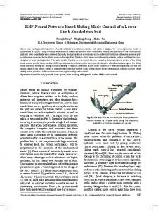
Online RBF and fuzzy based sliding mode control of robot manipulator Mohammed Salem

Mohamed Faycal Khelfi

RIIR Laboratory, Faculty of Sciences and Technology Mascara University Mascara, Algeria [email protected]

RIIR Laboratory, Faculty of Sciences University of Oran Oran, Algeria [email protected] we will update the gain of the corrective control using a fuzzy controller. Matlab Simulations are used to validate the RBF and fuzzy based sliding mode control applied to a two degree of freedom robot manipulator.

Abstract— The aim of this work is the combination of radial basis function networks (RBF) and fuzzy techniques to enhance the sliding mode controllers. In fact, three RBFs networks were used to estimate the model parameters and to respond to model variation and disturbances, a sequential training algorithm based on Kalman filter was implemented, and to eliminate the chattering effect, a fuzzy controller was designed. The hybrid sliding mode controller had shown a strong ability to get over noise and uncertainties. The former controller was used to control a two degree of freedom robot manipulator. Keywords-component; Fuzzy control, Kalman filter, Radial basis function, Robot manipulator, Sliding mode.

II.

A. Robot manipulator dynamic model The dynamic equation of a manipulator of N degrees of freedom [1] is given by:

M (q )q&& + C (q , q& )q& + G (q ) + f (q& ) = t

I. INTRODUCTION This Nowadays, Robot manipulators are used more and more in industrial fields to achieve complex and hard tasks [1]. The main problem is that Robots are strongly nonlinear multivariable systems and are usually object to load variation, uncertainties and disturbances which make it very hard to control them.

(1)

where t is the actuators couples vector, q , q& , q&& are position, velocity and acceleration vectors respectively. M(q) is the inertia matrix, it is symmetric and positive definite, C (q , q& ) is the is the Coriolis/centripetal nxn matrix while G(q) is the gravity nx1 vector. f (q&) is the friction terms vector: f (q& ) = K 1sgn (q& ) + K 2 q& , which is not taken into account in current work.

Sliding mode controllers try to drive the system states toward a specific surface and to slide over it [2], these controllers are robust to both structured and unstructured uncertainties but suffers from two major disadvantages. The first one is the existence of high frequency oscillation in the control signal 'chattering', and the other is the model dependency where the system parameters are needed to compute the equivalent control.

The robot dynamic (1) is strongly non-linear and complex to model B. Sliding mode control The sliding mode control is based on driving the robot states to slide over a surface s where all motion in neighborhood of the manifold is driven toward the manifold [7].

Radial basis function (RBF) neural networks with their approximation capabilities [3] [4], are able to estimate any complex nonlinear system parameters even in presence of disturbances especially using a sequential training algorithm and a growing and pruning strategy. Several researches tried to combine this technique with the fuzzy logic in robot manipulator sliding mode control. in [3], authors used a fuzzy controller to compute the gain K in the discontinuous control part while [6] trained one RBF network to estimate the global robot model function.

Let's define the tracking error like [7]:

e = q - qd

(2)

Where qd is the desired position and q is joint position. The sliding surface is defined by [2]:

To overcome the sliding mode control difficulties, in this paper we will use three RBF networks to estimate the model parameters in the equivalent control, these networks are trained using a modified sequential algorithm (Extended Minimal Resource allocation Network) and to eliminate the chattering

978-1-4673-1658-3/12/$31.00 ©2012 IEEE

PROBLEM FORMULATION

s = e& + le

(3)

where l=diag[l1, l2….ln], li is a positive constant.

896

We have to choose t so that the energy of the system will decay when s is not null so it has to satisfy the condition [7]:

1d 2 s i £ -h s i 2 dt

Equivalent

control

(4)

+-

s , s&

Corrective control

Robot

S

q d ,q&d ,q&&d

q ,q& ,q&&

t is chosen to be the sum of an equivalent control t eq and a corrective control t c (Fig. 1) [13]:

t = teq + t c

Figure 1. Sliding mode control

III.

(5)

A. Network description Radial basis function networks are a variety of artificial neural networks (RBF), it has one hidden layer and a linear ) ) ) ) output [3] y = [ y 1 , y 2 ,...., y ny ] (Fig. 2).

where

) ) ) t eq = M (q )q&&r + C (q , q& )q&r + G (q )

RADIAL BASIS FUNCTION NEURAL NETWORK

(6)

) y = FT (X ).A

and

t cc = -Ksign (s )

(7)

A is the weight's vector connecting the hidden layer to the output layer. FT (X ) is the response of the hidden layer to the input vector X=[1,x1,x2,…,xnx) where F is the Gaussian function given by:

) ) ) M , C , G are estimations of M, C, G respectively [7]. K=diag [K1, K2….Ki] is a diagonal positive definite matrix in which Ki is a positive constant and [13] q&&r = q&&d - le& and q&r = q&d - le

æ X -m F(X ) = exp ç ç s2 è

(8)

The system in closed loop is given by:

Ms& + Cs = Df - sign (s )

(9)

ö ÷ ÷ ø

(13)

B. Online Weights modification with Kalman filter To obtain the desired behavior, the neural network is trained using the Extended Minimal Resources allocation (EMRAN) where the RBF network begins with no hidden units, that is n = 0.[8], [9] As each input-output training data (xi, yi) is received, the network is built up based on three growth criteria [10]:

(10)

To prove the stability of the proposed controller we choose a Lyapunov function [7]:

1 V (s ) = s T Ms 2

2

m is the center's vector of the hidden neurons and s is the width of the Gaussian function.

where:

) ) ) Df = (M - M )q&&r + (C - C )q&r + (G -G )

(12)

x1

(11)

x2

The condition for the negativity of the derivation of V is that K has to be chosen inferior than the boundary of Df [2].

xnx

One of the main difficulties encountered in this control law is that it suffers from chattering phenomena due to the discontinuity of control signal (use of the sign function). The other one is that the designer has to know the exact mathematical model of the system to minimize the boundary of Df and so the value of K to cancel the effect of chattering, which is not always evident due to disturbances, friction and uncertainties.

F1(X)

a11

a1ny

S

) y1

F2(X)

an1 Fn(X)

S

) y ny

anny

Figure 2. Radial Basis Function Network Model

897

) e i = y i - y ( x i ) f E1

(14a)

0 ö æ Pi -1 Pi = ç ÷ è 0 q 0 I g *g ø

(14b)

ermsi =

i

e 2j

j = i - ( M -1)

M

å

f E2

d i = x i - mir f E 3

where the new rows and columns are initialized by q0(an estimate of the uncertainty when the initial values assigned to the parameters). The dimension g of the identity matrix I is equal to the number of new parameters introduced by the new hidden neuron.

(14c)

where μir is the center of the closest hidden unit to current input xi. E1, E2 and E3 are thresholds to be selected appropriately. Formula (14a) decides if the existing neurons are insufficient to obtain a network output that meets the error specification. Formula (14b) ensures the convergence of the sum squared error for the last M outputs. Formula (14c) checks if the added node is far from all existing neurons [9].

IV. FUZZY CONTROL Usually, a fuzzy system has one or more inputs and a single output with a rule base and an inference engine as showed in Fig. 3. The rules in the rule base are in the following form [14]: IF xi is Ai THEN yi is Bi where m Ai and Bi are fuzzy sets

1) Adding a new neuron: When all the criteria in (14) are met, a new hidden node is added. The new node has the following parameters [10]:

aN +1 = e i , mN +1 = x i ,s N +1 = k x i - mir

The output of the fuzzy controller is:

M

(15)

y =

κ is the overlap factor. 2) Updating the parameters using EKF If the criteria in (14) are not met, the network parameters w = [AT , mT , s T ] are updated using the extended Kalman filter (EKF) as follows [11], [12]:

w i = w i -1 + K i ei

åq Õ m

m =1 M

åÕ m =1

n i =1

n

i =1

mA (x i* ) m

i

(20)

mA (x ) * i

m

i

is

the

y membership

v (x ) = [v 1 (x ),...,v m (x ),....v M (x )]T is the vet or of heights of y membership functions and

(16)

Õ m (x ) (x ) = åÕ m (x ) n

v (17)

m

i =1

M

m =1

) ) B i = Ñw y is the gradient matrix of the function y

A

* i

m

i

n

i =1

A

m

i

and M is the amount of rules

* i

[14].

Ri is the variance of the measurement noise. Pi is the error covariance matrix which is updated by:

Pi = [I z *z - K i B iT B i ]Pi -1 + qI z *z

= q T v (x )

Where q = [q 1 ,..., q m ,....q M ]T functions centers vector.

where Ki is the Kalman gain matrix given by:

K i = Pi -1B i [Ri + B iT Pi -1Bi ]-1

(19)

Rule base

x

(18)

A Fuzzification

q is a scalar that determines the allowed random step in the direction of the gradient matrix. If the number of parameters to be adjusted is z, then Pi is a z × z positive definite symmetric matrix. When a new hidden neuron is added, the dimensions of Pi will be [10]:

Fuzzy inference engine

B

Figure 3. Fuzzy controller

898

y Defuzzification

V. RBF AND FUZZY SLIDING MODE CONTROL DESIGN To fix the problems of model depending and chattering of the sliding mode control in (5) we use artificial intelligence techniques: (6).

B. Fuzzy corrective control The corrective control in (7) is obtained by a fuzzy controller. The tuning rule for the gain K is to decrease its value near the sliding surface in order to damp the chattering amplitude and to increase it far from the surface. In this regard, a fuzzy controller rule base is proposed for tuning K as illustrated in table. 1, in which inputs are the surface s and it’s time derivative respectively. (ZE: Zero; B: Big; M: Medium; N: Negative; P: Positive). For multiple-output system, they can be considered as a combination of several single-output systems.

- Three RBF networks to estimate matrices M, C and G in - Fuzzy controller to get the appropriate values of K in (7). The resulted controller is showed in Fig. 4

A. RBF based equivalent control The main idea is to use RBF networks defined in section 2 to estimate the parameters of the equivalent control. The networks are rained online using EKF. In this work we use one RBF network to estimate inertia matrix M, another one to estimate matrix C and the last to estimate gravity vector G. The outputs of the RBF networks are the components of the matrices as shown in Fig. 5.

) M (q ) = FTM (X ).AM , X = [qT ]

VI. SIMULATION RESULTS Simulations were carried out over two degrees of freedom robot manipulator whose dynamic model is given by (24) [15]:

M (q )q&& + C (q , q& )q& + G (q ) = t with:

(21)

) C (q , q& ) = FTC (X ).AC , X = [qT , q&T ]

(22)

) G (q ) = FTG (X ).AG , X = [qT ]

(23)

é0.77 + 1.02cos( q2 ) 0.76 + 0.51cos( q2 ) ù M (q ) = ê ú 0.62 ë0.76 + 0.51cos( q2 ) û

é -0.5sin(q ) q. . 2 2 C ( q, q) = ê . ê ëê 0.5sin(q2 ) q1

RBF control

+-

s , s&

Robot

S

q d ,q&d ,q&&d

q&&r

To accomplish the control, we started by choosing the appropriate membership function for the surface s, its derivation and the gain K to compute the corrective controller. Membership function of s and ds are in Fig. 6 and Fig. 7

x

) M

) G

S

teq

TABLE I.

x

q& C%

(25)

We used the sliding mode control in (5) to control the two dof robot manipulator and to test the robustness of the controller, we added a white noise to the output of robot after the time 0.2 and changed the parameters of the inertia matrix by altering the mass of link one.

Figure 4. RBF and fuzzy sliding mode controller

q

. . -0.5sin(q2 )( q1 + q2 ) ùú ú 0 ûú

é7.6sin(q1 ) + 0.63sin(q1 + q2 ) ù G( q) = 10 ê ú 0.63sin(q1 + q2 ) ë û

q ,q& ,q&&

Fuzzy control

(24)

N Z P

q&r

Figure 5. RBF based equivalent controller

899

s&

s

FUZZY RULE BASE FOR TUNING “K”

NB

NS

ZE

PS

PB

KB KB KB

KB KM KS

KM KS KM

KS KM KB

KB KB KB

1

NB

NS

ZE

PS

Fig. 11 and Fig. 12 show the position error of the robot joints and Fig. 13 and Fig. 14 present the velocity errors. We see that errors are acceptable even a white noise is present and some uncertainties in inertia matrix.

PB

De g re e of m em b e rs h ip

0.8 0.6 0.4

Values of the gain K are presented in Fig. 15 and it is clear that K is big far from the surface and when the system states are close to the sliding surface the values of k are decreased to be null.

0.2 0 -1

-0.8

-0.6

-0.4

-0.2

0

0.2

0.4

0.6

0.8

1

S urfac e s

Figure 6. Membership function of s

N

1

Z

Fig. 16 presents the torques acting on the robot joints where the absence of chattering could clearly be seen.

P

D eg r ee o f m e m b ersh i p

0.8

15

x 10

-3

0.6 0.4

E rr o r in p o s it i o n j o i n t 1

10

0.2 0 -1

-0.8

-0.6

-0.4

-0.2

0

0.2

0.4

0.6

0.8

1

S urface d eriva tive ds

Figure 7. Membership function of Ds

0.1

0.2

0.3

0.4

0.5

0.6

0.7

0.8

0.9

1

0.8

0.9

1

0.8

0.9

1

Time(s)

Figure 11. Position errors of joint 1 15

x 10

-3

10

-5

p o s it io n e rr o r jo in t 2

in e rt ia m a t ri x R B F e rro r

x 10

0 -5 0

For the equivalent control, the three RBF networks are trained using the EMRAN algorithm. Errors of networks are in Fig. 8, Fig. 9 and Fig. 10. Due to the performance of the training algorithm, estimation errors are about 10-5, 10-6 and 10-3 for the three RBF networks. 15

5

M(1,1) error M(1,2) error M(2,1) error M(2,2) error

10

5 0

5

-5 0

0

0.1

0.2

0.3

0.4

0.5

0.6

0.7

Time(s)

-5 0

0.1

0.2

0.3

0.4

0.5

0.6

0.7

0.8

0.9

Figure 12. Position errors of joint 2

1

Time(s)

Figure 8. RBF estimation errors of inertia matrix x 10

4

0.02

-6

C(1,1) error C(1,2) error C(2,1) error C(2,2) error

0 v e l o c i t y e r r o r j o in 1

C o ri o li s R B F e r ro r

2

-0.02

0

-0.04

-2

-0.06

-4 0

0.1

0.2

0.3

0.4

0.5

0.6

0.7

0.8

0.9

-0.08 0

1

Time(s)

0.1

0.2

0.3

0.4

0.5

0.6

0.7

Time(s)

Figure 9. RBF estimation errors of Coriolis matrix

Figure 13. Velocity errors of joint 1

-3

5

x 10

G ra v i t y R B f e r ro r

0 -5

G(1) error G(2) error

-10 -15 -20 0

0.1

0.2

0.3

0.4

0.5

0.6

0.7

0.8

0.9

1

Time(s )

Figure 10. RBF estimation errors of gravity vector

900

REFERENCES

0.02

[1]

v e lo c it y e r ro r j o i n 2

0

[2] [3]

-0.02 -0.04

[4]

-0.06 0

0.1

0.2

0.3

0.4

0.5

0.6

0.7

0.8

0.9

1

[5]

Time(s)

[6] Figure 14. Velocity errors of joint 2 [7] 40

K g a in v a ri a t i o n

30

[8]

K1 for first join K2 for second join

20 10

[9]

0

-10

[10]

-20 0

0.1

0.2

0.3

0.4

0.5

0.6

0.7

0.8

0.9

1

Time(s)

[11] [12]

Figure 15. Gain K variations

[13] 100

T o r q u e o n jo i n t 1 a n d 2

[14]

Joint 1 Joint 2

50

[15]

0 -50

-100 0

0.1

0.2

0.3

0.4

0.5

0.6

0.7

0.8

0.9

1

Time(s)

Figure 16. Control signal

VII. CONCLUSION We presented in this paper a sliding mode controller for robot manipulator where the equivalent control was achieved using three radial basis function neural networks to estimate the robot matrices. A modified version of the sequential training algorithm EMRAN was used. The corrective control was replaced by a fuzzy controller to compute the K gain values along the control. The obtained results seem to be good and we avoided the classical sliding mode problems by canceling the chattering in the control signal and the estimation of model parameters.

901

F.L Lewis, , C. T. Abdallah, and D. M. Dawson , Control of Robot Manipulators, Macmillan Publishing Company, Inc, USA, 1993. J.E. Slotine, W.Li, Applied Nonlinear control, Prentice Hall S. Haykin, Neural Networks: A Comprehensive Foundation. Upper Saddle River, N.J.: Prentice Hall, 1999. 2nd Edition. D. Broomhead and D. Lowe, “Multivariate function approximation and adaptive networks,” Complex Systems, vol. 2, pp. 321–355, 1988. S.E. Shaffei, "Sliding mode control of robot manipulators via intelligent approaches, in: Advances strategies for Robots manipulators". Sciyo, vol.172,pp 135, 2010. A. G. Ak, and G. Cansever, “Sliding mode controlller with rbf networks for robotic manipulator trajectory tracking,” Lecture notes in control and information sciences (Intelligent Control and Automation ), vol. 144, 1981, pp. 527–532. A. Bagheri, M.A. Roudbari and M.J. Mahmoodabadi, "Adaptive and Sliding Mode Control for Non- Linear Systems", Int J Advanced Design and Manufacturing Technology,2010 , Vol. 3/ No. 4. N. Sundararajan, P. Saratchandran, and L. Yingwei, “Radial basis function neural networks with sequential learning: MRAN and its applications,” River Edge: Singapore;World Scientific: NJ, 1999. G.B. Huang, P. Saratchandran and N. Sundararajan, "A Generalized Growing And Pruning RBF(GGAP-RBF) Neural Network for Function Approximation", IEEE Trans. on Neural Networks, 2004. Y. Li, N. Sundararajan, P. Saratchandran, "Analysis of Minimal Radial Basis Function Network Algorithm for Real-Time Identification of Nonlinear Dynamic Systems, Control Theory and Applications", IEE Proceedings, 2000. B. Anderson, J. Moore, Optimal Filtering, Prentice-Hall, Englewood Cli4s, NJ, 1979. D.Simon, "Training Radial Basis Neural Networks with the Extended Kalman Filter". Neurocomputing 48 (2002) 455-475. T.P. Leung, C.-Y. Su, Q.-J. Zhou, "Sliding mode control of robot manipulators: a case study", Industrial Electronics Society, IECON '90, 1990 W. Li, X. G. Chang, F. M. Wahl, and J. Farrell, “Tracking control of a manipulator under uncertainty by fuzzy P+ID controller,” Fuzzy Sets Syst., vol. 122, no. 1, pp. 125–137, 2001. M.F. Khelfi, M. Zasadzinski, H. Rafaralahy, E. Richard, and M. Darouach (1996), "Reduced-order observer-based point-to-point and trajectory controllers for robot manipulators", A Journal of IFAC the International Federation of Automatic Control. Vol. 4, N° 7, pp. 9911000, 1996 Elsevier Science ltd,