Online System-Identification Using Subspace Algorithms for the

2008 American Control Conference Westin Seattle Hotel, Seattle, Washington, USA June 11-13, 2008

FrB04.3

Online System-Identification Using Subspace algorithms for the control of Microscopic processes Antonios Armaou†,∗

Sivakumar Pitchaiah Abstract— The problem of online system identification and control of microscopic processes is considered. Traditionally, such processes are numerically simulated employing atomistic simulations. The unavailability of closed-form models to describe the evolution makes the controller design task challenging. A methodology is developed in which subspace algorithms for bilinear system identification are coupled with feedback linearization techniques with objective the online identification and control of microscopic processes. We illustrate the applicability of the proposed methodology on a Kinetic Monte Carlo (KMC) realization of a simplified surface reaction scheme that describes the dynamics of CO oxidation by O2 on a Pt catalytic surface. The proposed controller successfully forces the process from one stationary state to another state.

I. I NTRODUCTION Owing to a competitive global market and reduced profit margins, recent focus in the microelectronics industry has been towards tighter quality control based on device performance specifications. To achieve such a goal, the properties of the end product microstructure need to be characterized. As a result, we need models for microelectronics fabrication processes that take in to account events that take place at disparate time and length scales, (namely, the process scales of seconds and the product ones of nano seconds). Such models, which also describe many chemical, biological and material process systems, are called multiscale systems and pose significant challenges both from an analysis and control point of view [3]. These difficulties can be attributed in part to the unavailability of closed form descriptions of the microscopic process evolution. Motivated by this, a significant amount of research has been focused on the development of control methods to overcome these difficulties. One of the proposed approaches designed feedback controllers by employing Kinetic-Monte-Carlo (KMC) simulations as the underlying process observer [12]. It was successfully applied to regulate the surface roughness in a GaAs deposition process model [13]. Since the KMC models are not available in closed form, the design of modelbased controllers was impossible. Taking this into account in [14], [16], controllers were designed using the linearized Kuramoto-Sivashinsky equation (KSE) as the underlying process model. To improve on the linear controllers an extension was proposed in [15], where the authors designed a nonlinear feedback controller to control the roughness of a one dimensional surface again employing stochastic † Dept. of Chemical Engineering, The Pennsylvania State University, University Park, PA 16802, Tel: (814) 865-5316, Email:

[email protected] ∗

corresponding author

978-1-4244-2079-7/08/$25.00 ©2008 AACC.

KSE as the underlying process growth model. The proposed approach assumed a specific structure to the nonlinear stochastic terms. In [19] linear models were identified directly based on the output from KMC simulators. The linear controller that was designed based on the identified model, was used to control the lower order statistical moments of microscopic distributions. In a different approach [22] the problem of non availability of closed form models was addressed by deriving a low-order state space model through offline system identification, based on finite set of ”coarse” observables. The identified state space model was used to design a receding horizon controller to regulate the roughness, during thin film growth, at a particular setpoint. The coarse observables in this work were identified from spatial correlation functions of the thin film surface to represent the dominant traits of the microstructure during a deposition process. In [24] it was shown that the different deposition surfaces, constructed through a stochastic reconstruction procedure, with identical values of these variables exhibited approximately identical coarse dynamic behavior. In a different approach [8] a methodology based on proper orthogonal decomposition and in [17] a data driven approach, were developed for the statistical reduction of the master equation. Another approach [20] deals with the feedback linearization problem of nonlinear systems described by microscopic/ stochastic simulators, in which the non availability of a closed form model was circumvented by directly calculating the quantities needed for design of nonlinear controllers from appropriately initialized microscopic simulations. A shortcoming of this method however is that it is limited to stabilization and involves closed loop eigenvalue assignment constraints. In [1], [23] the so called hybrid multiscale process models were used, where the continuum laws which are applicable at the macroscopic level were combined with computationally expensive microscopic laws (Monte-Carlo (MC) / KMC or Molecular dynamics (MD)) to get the ”coarse” process behavior. Using the ”coarse” variables nonlinear process models were identified offline through the solution of a series of nonlinear programs. Subsequently the identified models were used to design output feedback controllers. The methodology used in this approach is computationally intensive and involves offline process identification. The present work deals with the online identification of nonlinear models that accurately describe the evolution of the process output based on information from microscopic simulations. We build upon the approach of [1], [22] and de-

4413

velop a computationally tractable online process model identification and adaptive control methodology, which takes into account the change in the underlying process dynamics as the process traverses different regions in the variable state space. The computationally tractable online system-identification component of the approach is based on subspace-system identification (SSI). SSI algorithms [6], such as N4SID are traditionally used to identify linear systems. Recently, N4SID was also extended for identification of bilinear systems excited by white inputs [6]. A modification for bilinear systems excited by general inputs was also proposed in [4]. We extend the applicability of SSI algorithm to identify a nonlinear process model and subsequently design output feedback linearizing controllers based on the identified model. The process model is updated as new measurements become available, to better approximate the microscopic process evolution. We illustrate the applicability of the proposed identification scheme on a Kinetic Monte Carlo (KMC) realization of a simplified surface reaction scheme describing the oxidation of CO by O2 on a Pt catalytic surface [2]. Employing the proposed methodology we design an output feedback controller that successfully forces the process from one stationary state to another. This paper is organized as follows. In subsection II-A we present concepts from Carleman linearization that show that a nonlinear, affine in input model can be approximated by a discrete time bilinear model. In subsection II-B the system identification technique adopted is presented. In section III an output feedback controller is designed based on the identified bilinear model. In section IV the methodology for online identification of microscopic processes is presented; in section V an example is presented to illustrate the methodology. II. M ATHEMATICAL FORMULATION We seek to identify nonlinear dynamic models of nonlinear dynamic systems with the following state space representation x˙ = f (x) + g(x)u, x(0) = x0 (1) where x ∈ IRn is the vector of state variables, u ∈ IR is a scalar input. f (x) is a nonlinear vector function of the state, and g(x) is a nonlinear vector function which accounts for the influence of the control actuator on the process. We assume that the functions f(·) and g(·) are analytic in their arguments and that we have full state information of the process available. Moreover, without loss of generality, we also assume that the target steady state of the system is the origin. In the remainder of this manuscript we use the following notation, where the Kronecker product between matrices A ∈ IRN×M and B ∈ IRL×K can be defined as a matrix C ∈ IR(NL)×(MK)   a1,1 B a1,2 B · · · a1,M B  a2,1 B a2,2 B · · · a2,M B   C = A⊗B ≡  (2)  ··· ··· ··· ···  aN,1 B aN,2 B · · · aN,M B

We also define the k-th order Kronecker product as A[k] = A[k−1] ⊗ A, A[1] = A and A[0] = 1. In ∈ IRn×n is defined as the unitary matrix of dimension n. The Khatri-Rao product for two matrices A = [a1 , a2 , ..., am ] ∈ IRr×m and B = [b1 , b2 , · · · , bm ] ∈ IRs×m is defined as the column-wise Kronecker product A ⊙ B = [a1 ⊗ b1 , a2 ⊗ b2 , · · · , am ⊗ bm ] ∈ IRsr×m . The orthogonal projection of the row space of matrix A ∈ IRr×m into the row space of matrix B ∈ IRs×m is defined as A/B = AB† B. The Moore-Penrose pseudoinverse of a matrix A ∈ IRr×m is a matrix A† ∈ IRm×r such that AA† A = A.

A. Problem formulation Referring to the system of (1), we apply McLaurin series expansion to the nonlinear vector fields f (x), g(x), to obtain ∞

f (x) =

∞

1

1

∑ k! f[k] |x=0 x[k] ; g(x) = g(0) + ∑ k! g[k] |x=0 x[k]

(3)

k=1

k=1

k

k

where f[k] |x=0 ∈ IRn×(n ) and g[k] |x=0 ∈ IRn×(n ) are the kth partial derivatives of f (x) and g(x) with respect to x, respectively, evaluated at x = 0. To simplify the notation we denote Ak ≡ (1/k!) f[k] |x=0 , Bk ≡ (1/k!)g[k] |x=0 , ∀k and B0 = g(0) for the rest of the paper. With x[k] we denote the kth Kronecker product, and (·)! denotes the standard factorial of integer (·). Thus, (1) can be equivalently written in the form x˙ = f (x) + g(x)u ≡

∞

∞

k=1

k=0

∑ Ak x[k] + ∑ Bk x[k] u

(4)

We will focus on a finite order polynomial approximation of the nonlinear system of order p f for f (x) and pg for g(x). Without loss of generality we assume that p f = pg + 1 = p, in which case (4) takes the form: p

x˙ ≃

p−1

∑ Ak x[k] + ∑ Bk x[k] u k=1

(5)

k=0

To linearize the system of (4), we compute the dynamic behavior of the terms x[k] as follows: p−k d(x[k] ) p−k+1 = ∑ Ak,i x[i+k−1] + ∑ Bk,i x[i+k−1] u dt i=1 i=0 k−1

where Ak,i = larly.

[l]

∑ In

[k−1+l]

⊗ Ai ⊗ In

(6)

and Bk,i is defined simi-

l=0 T

T

Defining x⊗ = [xT x[2] · · · x[p] ]T , the system of (6) can be written in the following bilinear form

4414

x˙⊗ = A x⊗ + [N u⊗ x + B u]

(7)

where A , N and B are matrices of the form:    A1,1 A1,2 · · · A1,p B1,0  0   A · · · A 2,1 2,p−1    0   0 0 0 · · · A A = , B = 3,p−2     ···  ··· ··· ··· ···  0 0 ··· A p,1 0   N1,1 N1,2 · · · N1,p−1 0  N2,0 N2,1 · · · N2,p−2 0    N3,0 · · · N3,p−3 0  N =   0  ··· ··· ··· ··· ···  0 0 ··· N p,0 0

Y p|q = [Yp Y p − 1|q U p ⊙Y p − 1|q]T , Y q|p = [Yq Y q + 1|p Uq ⊙Y q + 1|p]T , Yp = [y(p) y(p + 1) · · · y(p + j)],



  ,  

for p ≫ q and j ≫ p, q. U p is defined similarly to Yp . The parameter i should be chosen such that di−1 = p−1 l > n where l is the number of outputs. ∑i−1 p=1 (m + 1) 2) Compute the singular value decomposition (SVD) of µ ¶µ T ¶ S1 0 V1 Oi = (U1 U2 ) (13) 0 S2 V2T where S1 ∈ IRn×(n) , and Γi and Xˆi are defined as Γi = 1/2 1/2 U1 S1 , Xˆi = S1 V1 3) Calculate the estimated state vector sequence at time step i+1 as: Xˆi+1 = Γ†i−1 Oi+1 , Γi−1 = [γTl+1 γTl+2 , · · · ]T where γ1 , γ2 ,· · · are the rows of Γi 4) Obtain the system matrices by solving the following linear least squares problem:

(8) The presented operation, also known as Carleman linearization [11], sets the basis for the identification of the system behavior. Time discretization of (7) with piece-wise constant control action u(t) = u(kTˆ ), kTˆ ≤ t ≤ (k + 1)Tˆ , (where Tˆ is the sample time) leads to [18]: ∞

∞

x((k + 1)Tˆ ) = Ax(kTˆ ) + ∑ Ni u[i] ⊗ x(kTˆ ) + ∑ Bi u[i] (kTˆ ) i=0

i=0

(9)

where A, Ni ,Bi are defined as ˆ

A = eA T Z Tˆ

Ni =

Z0

eA (T −σ1 ) N

Z σ1

eA (σ1 −σ2 ) N · · ·

0 σi−1 A (σi−1 −σi )

N eA σi dσi dσi−1 · · · dσ1

e

0

Z Tˆ

Bi =

eA (T −σ1 ) N

Z0 σi−1

e

Z σ1

eA (σ1 −σ2 ) N

(10)

···

B dσi dσi−1 · · · dσ1

Truncating the infinite series up to order q and assuming Tˆ = 1 for convenience, we obtain the following bilinear discrete time system of form x(k + 1) = Ax(k) + Nu⊗ (k) ⊗ x(k) + Bu⊗ (k)

Xˆi+1 Yi |i

¶

µ

A C

N 0

B 0

¶



X(k + 1) = AX(k) + Nu(k) ⊗ X(k) + Bu(k) x(k) = CX(k)

0 A (σi−1 −σi )

0

 µ ¶ Xˆi ρw   ˆ Ui ⊙ Xi = + ρv Ui (14) known parameterizations of the matrices A, B, N and C can be easily handled by solving the above problem as a constrained linear least squares problem. The state space models obtained from the subspace algorithm can be written as: µ

(11)

where u⊗ = [u[1] , u[2] , · · · , u[q] ], N = [N1 , N2 , · · · , Nq ] and B = [B1 , B2 , · · · , Bq ]. This discrete-bilinear model approximates (up to arbitrary accuracy) the nonlinear model of (11). In this work q is taken to be 4.

(15)

Where X(k) ∈ IRq× j are the states used in system identification. The output of system-identification component can be thought of as linear combination of states, X(k), which by themselves do not have any physical interpretation. One important assumption is that the process is noiseless. Even though this appears to be restrictive we show that feedback controller designed on the basis of the identified model from the stochastic simulation algorithm forces the process to reach the desired set point. Remark 2.1: We note that if we have previous knowledge of structure for the system of (1), we can take advantage of the information in the presented methodology seamlessly through the use of Lagrange expansions in (3).

B. System Identification We now use bilinear subspace system-identification for white inputs [5] to identify (11). For the sake of completeness we briefly outline the algorithm as following: 1) Compute the projections · ¸ Yi−1 |0 Oi = Yi |2i−1 / Ui−1 · |0 ¸ (12) Yi |0 Oi+1 = Yi+1 |2i−1 / Ui |0 where

III. O UTPUT FEEDBACK CONTROLLER BASED ON FEEDBACK LINEARIZATION

Once the model for the system of (1) is identified as illustrated in the previous section, we employ the feedback linearization technique of [21] to force a linear closed loop behavior to the system. The relative degree of the model we obtain from system identification (15) is 1 i.e. the input affects the output from the system after one time period. We note that the relative degree of the original system of (1) need not be 1. The underlying assumption is only that the

4415

relative degree is finite, which then will be captured by the proposed representation. The desired input /output behavior to the closed loop system is of the form x(k + 1) = (1 − λ)xsp + λx(k)

(16)

The desired closed loop response is chosen to make the system progress towards the desired setpoint smoothly. Clearly the control action which achieves the above closed loop behavior is of the form: u(k) = (CNX +CB)−1 (−CAX(k) + λx(k) + (1 − λ)xsp ) (17) where λ is a tuning parameter such that 0 < λ < 1. The error dynamics of the closed loop system of (16) is given as e(k + 1) = λe(k) where e(k) = x(k) − xsp The choice of the control parameter, λ plays an important role in deciding how fast the controller forces the processes towards its setpoint. This can be clearly seen from (16). For values of λ close to 1, the output converges to the setpoint slowly. On the other hand, for values of λ close to 0 the control action is large leading to fast convergence of the output to the setpoint. However in this case the system matrices obtained from the system identification will be ill conditioned, since the bilinear models cannot capture a rapid change in the process behavior, if the frequency of the measurements is not appropriately adapted. IV. O NLINE SYSTEM IDENTIFICATION AND CONTROL ALGORITHM

We are now ready to present the methodology for identification and control. The method consists of the following steps. • Perturb the system in the neighborhood of the Initial stationary state using an input sequence (described in Remark 4.2) excited by a Gaussian noise and obtain the output sequence. •

Identify a bilinear model of the form in (15) at the initial stationary state using the system identification algorithm of subsection II-B.

•

Calculate the necessary control action from (17) to force the system to a new stationary state towards the desired setpoint.

•

Identify the system at the new stationary state by employing the new input signal obtained using the calculated control action as carrier signal to obtain an output sequence.

•

Augment the new input/output sequence to the previous available sequence. Employ a window of size nˆ truncate older data to obtain a sequence containing nˆ entries

•

Repeat steps 2 − 4 until the desired setpoint is reached.

Remark 4.1: With the addition of the new sequence to the previous data, the oblique projection matrices need only to be augmented. Thus some computational savings are gained Remark 4.2: Since the system identification algorithm as described in the subsection II-B requires the input to persistently excite the system in the neighborhood of the current state, we generate the input sequence by perturbing a carrier signal (which may be our control signal), using a gaussian white noise. V. I LLUSTRATIVE EXAMPLE : CO OXIDATION A. problem formulation We illustrate the online system identification and control methodology presented in the section IV on a KMC realization (using the stochastic simulation algorithm [9],[10]) of a simplified reaction model of the form A + 21 B2 −→ AB of CO oxidation by O2 on Pt catalytic surface. The process involves adsorption of A, dissociative adsorption of B2 , and a second-order surface reaction whose products desorb immediately. The mean-field Langmuir-Hinshelwood approximation equations for this process in the absence of adsorbate interaction would consist of a set of two ODES [2]. d(θA ) = α(1 − θA − θB ) − γ(θA ) − 4kr θA θB dt

(18) d(θB ) 2 = 2β(1 − θA − θB ) − 4kr θA θB dt where θA , θB represent the surface coverage of CO, and O2 , respectively, α, β are the rate constants for adsorption of CO and O2 , respectively, γ is the rate constant for CO desorption and kr is the reaction rate constant. We employed β as the manipulated input. The values of these parameters are taken to be α = 1.6, γ = 0.04 and kr = 1. The above model exhibits two turning points for the value of parameter β ≈ 2.5 and 8.49 [2]. This work employs only an atomistic realization of the above process (18) to identify and control it. The probability of lattice being at a particular configuration is given by the master equation [7] d(P(σ,t)) = ∑ W (σ′ → σ)P(σ′ ,t) − ∑ W (σ → σ′ )P(σ,t) dt σ′ σ′ (19) where σ and σ′ are the probabilities of the lattice being at a particular configuration. KMC provides the numerical solution to the master equation, by randomly choosing one among various possible transition events (the transition events in our case are adsorption, desorption and the surface reaction at the catalyst surface) depending upon the event probabilities. These KMC simulations provide us with the expected behavior of the process and we use system identification to identify the underlying closed form model consistent with the realization provided by the KMC simulation. Design of controllers based on KMC simulations is challenging since a closed-form dynamic model is unavailable

4416

0.25

0.14

0.12

0.2 0.1

0.15

θ

θA

A

0.08

0.06

0.1 0.04

0.05 0.02

0 0

50

100

150

200

250

300

350

400

450

0 0

time(sec)

1000

1500

2000

2500

3000

time(sec)

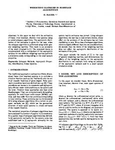
Open loop simulation of KMC for β = 5.6.

Fig. 2. Evolution of θA as the system evolves towards the desired stationary state. The dotted line represents the desired setpoint and the solid line represents the evolution of the process.

and KMC simulations reach the solution by probabilistically sampling the master equation. A further complication is that the physical size of the simulated catalytic surface and the number of times the process is simulated using KMC has an affect on the variance as well as the expectation of the output. As the size of the lattice increases the expected behavior of the stochastic process converges to the expected behavior described by the ODE system [9]. In this work the lattice size is chosen such that the discrepancy between the expected behavior obtained from KMC simulations and the ODE solutions are negligible [7]. Specifically, we used KMC with a lattice size of 100 × 100 sites and an average of 100 runs was used to compute the expected process behavior. The reporting horizon was chosen to be 0.8 sec. Figure 1 shows a sample open loop KMC simulation of the CO oxidation model, with β = 5.6. It is observed that the KMC simulations are inherently associated with noise. We show in the next section that even though we do not explicitly consider noise while designing the controller, the closed-loop system is ultimately forced by the controller to reach its desired setpoint. Remark 5.1: The computational time for each KMC simulation with an input sequence of length 1000 is 50 sec of CPU time. CPU time for identification of each bilinear model is 3 sec. This time can be significantly improved by using new techniques to compute SVD of the projection matrix Oi . B. Results and Discussion Our objective was to dynamically force the system from an initial stationary state to a desired stationary state. Specifically, our objective was to increase the surface coverage (θA ) of CO on the catalytic surface from 0.06 to a desired value of 0.2. To achieve the desired objective we use the online system identification and control methodology as presented in section IV. The tunable parameter λ of the controller was set to 0.96. It can be observed from figure 2 that the controller combined with online system identification scheme is able to drive the system to the desired objective. Specifically, the controller acted on the error between the desired setpoint

5.5

5

4.5

u

Fig. 1.

500

4

3.5

3

0

500

1000

1500

2000

2500

time(sec)

Fig. 3. Control effort that drives the system towards the desired stationary state.

and the current value of the θA to force the system towards the desired objective. The fluctuations observed during the evolution of θA can be attributed to the stochastic nature of the microscopic system. The increase in the magnitude of the fluctuations observed in θA in figure 2 (similarly in θB in figure 4) as the system evolved towards the desired stationary state is due to the fact that the system is being forced to a region close to the bifurcation point, where the rate of change of output with a small change in input is high. Our aim was to the force θA to reach a particular setpoint; the change in θB , seen in figure 4 can be attributed to the coupling in the dynamics of θA and θB , as observed from the deterministic steady state bifurcation diagram presented in [2]. Even though the output signal that we obtain from the KMC simulation and use for the identification contains noise (due to the stochastic nature of the system), we observe that the controller achieves forcing the system to the desired coverage value, even though it is not explicitly designed to account for noise. This is due to the identification scheme which filters to a large extend the effects of noise when computing the system (15). In future work we will employ

4417

0.8 0.7 0.6

θB

0.5 0.4 0.3 0.2 0.1 0 0

500

1000

1500

2000

2500

time(sec)

Fig. 4. Evolution of θB as the system evolves towards the desired stationary state.

0.12

0.1

θ

A

0.08

0.06

0.04

0.02

0 0

500

1000

1500

2000

2400

time(sec)

Fig. 5.

Evolution of θA after a step disturbance in reaction rate constant

the information by the identification algorithm to design robust controllers that explicitly account for the noisy signal. Finally, we studied the robustness of the controller in the presence of disturbances. Figure 5 presents the regulatory performance of the controller to a step change in the reaction rate constant of the reaction, kr from 1 to 2. It can be observed from the output profile that the effects of this parametric disturbance are rejected and the output again converged to the desired value. ACKNOWLEDGEMENTS Financial support from National Science Foundation, CAREER Award #CBET 06-44519 and the American Chemical Society - Petroleum Research Fund, Research Initiation Award #PRF 44300-G9 is gratefully acknowledged.

[4] W. FAVOREEL, Subspace methods for identification and control of linear and bilinear systems, PhD thesis, Katholieke Universiteit Leuven, Belgium. [5] W. FAVOREEL , B. D. M OOR , AND P. V. OVERSCHEE, Subspace identification of bilinear systems subject to white inputs, IEEE. Transactions on Automatic Control, 44 (1999), pp. 1157–1165. [6] , Subspace state space system identification for industrial processes, Journal of Process Control, 10 (2000), pp. 149–155. [7] K. A. F ICHTHORN AND W. H. W EINBERG, Theoretical foundations of dynamical Monte Carlo simulations, J. Chem. Phys., 95 (1991), pp. 1090–1096. [8] M. A. G ALLIVAN AND R. M. M URRAY, Reduction and identification methods for markovian control systems, with application to thin film deposition, Int. J. Robust & Nonlin. Contr., 46 (2004), pp. 269–282. [9] D. T. G ILLESPIE, A general method for numerically simulating the stochastic time evolution of coupled chemical reactions, J. Comp. Phys., 22 (1976), pp. 403–34. [10] , Exact stochastic simulation of coupled chemical reactions, J. Phys. Chem., 81 (1977), pp. 2340–2361. [11] K. L. KOWALSKI AND W.-H. S TEEB, Nonlinear Dynamical Systems and Carleman Linearization, World Scientific Publishing Company, Singapore, 1991. [12] Y. L OU AND P. D. C HRISTOFIDES, Estimation and control of surface roughness in thin film growth using kinetic Monte-Carlo methods, Chem. Eng. Sci., 58 (2003), pp. 3115–3129. [13] , Feedback control of surface roughness of GaAs (001)thin films using kinetic Monte Carlo models, Comp. & Chem. Eng., 29 (2004), pp. 225–241. [14] , Feedback control of surface roughness using stochastic PDEs, AICHE Journal, 51 (2005), pp. 345–352. [15] , Nonlinear feedback control of surface roughness using a stochastic PDE: Design and application to a sputtering process, Ind. Eng. Chem. Research, 45 (2006), pp. 7177–7189. [16] D. N I AND P. D. C HRISTOFIDES, Multivariable predictive control of thin film deposition using a stochastic PDE model, Ind. Eng. Chem. Research, 44 (2005), pp. 2416–2427. [17] C. O GUZ AND M. A. G ALLIVAN, A data-driven approach for reduction of molecular simulations, Int. J. Robust & Nonlin. Contr., 46 (2005), pp. 727–743. [18] E. A. RODRIGUES AND T. A. W EISSHAAR, Nonlinear discrete-time state-space modeling of dynamic systems for control applications, American Institute of Aeronautics and Astronautics, (1995). [19] C. I. S IETTOS , A. A RMAOU , A. G. M AKEEV, AND I. G. K EVREKIDIS, Microscopic/stochastic timesteppers and coarse control: a kinetic Monte Carlo example, AIChE J., 49 (2003), pp. 1922– 1926. [20] C. I. S IETTOS , I. G. K EVREKIDIS , AND N. K AZANTIS, An equationfree approach to nonlinear control: Coarse feedback linearization with pole-placement, Int. J. Bifurcation and Chaos, 16 (2006), pp. 2029– 2041. [21] M. S OROUSH AND C. K RAVARIS, Discrete-time nonlinear controller synthesis by input/output linearization, AICHE Journal, 38 (1992), pp. 1923–1945. [22] A. VARSHNEY AND A. A RMAOU, Feedback control of surface roughness during thin-film growth using approximate low-order ode model, in Proceedings of the 45th IEEE Conference on Decision and Control. [23] , Multiscale optimization using hybrid PDE /KMC process systems with applications to thin film growth, Chem. Eng. Sci., 60 (2005), pp. 6780–6794. [24] , Identification of macroscopic variables for low-order modeling of thin-film growth, Ind. Eng. Chem. Research, 45 (2006), pp. 8290–8298.

R EFERENCES [1] A. A RMAOU, Output feedback control of dissipative distributed process via microscopic simulations, Comp. & Chem. Eng., 29 (2005), pp. 771–782. [2] A. A RMAOU AND I. G. K EVREKIDIS, Equation-free optimal switching policies for bistable reacting systems, Int. J. Robust & Nonlin. Contr., 15 (2005), pp. 713–726. [3] P. D. C HRISTOFIDES AND A. A RMAOU, Control of multiscale and distributed process systems-preface, Comp. & Chem. Eng., 29 (2005), pp. 687–688.

4418