Online Topological Mapping of a Sparse Camera Network

Online Topological Mapping of a Sparse Camera Network Paulo Freitas1, Paulo Menezes1, Jorge Dias1, 1

Institute of Systems and Robotics, University of Coimbra, 3030-290 Coimbra, Portugal {pfreitas, paulo, jorge}@isr.uc.pt

Abstract. This article presents a method that without any prior knowledge of a network of cameras, in an automatic and in an on-line mode, estimates their positional relation. The developed method is also able to adapt the estimation of the topology automatically, if some change is made on the network, as adding or removing cameras, and changing the position relative to the adjacent ones. To compute the topological map of a sparse network of cameras, our approach registers events, generated by the entrance and exit of agents (persons or movable objects) from the visible area of the cameras. These events are classified as IN and OUT respectively, and they are stored and associated according to a predefined logic based on the measured entropy level of the overall of events, and joined in relation groups. These groups are then analyzed to infer the topological map. However, it is necessary to develop approaches to avoid and eliminate redundancy of data and remove false relations between the sensors. By this, to achieve reliable results and to prevent loss of data, a method is proposed to adjust the computation of the acquired data based on the entropy evaluation. Then, two algorithms are used to combine the events and to create the relation groups at predefined levels of entropy. Based on the categorization of the relation of the events and groups, is possible to estimate the topological information of sparse networks of cameras. Our experimental results show that, even in situations where there is a significant disorder in the registered events, our method is robust and performs valid estimations. Keywords: Sparse Network; Topological Map; Events; Calibration; Field of View.

1 Introduction The increase of size, complexity and with the integration of many devices into networks of cameras, or even considering multi-modal networks of sensors, the information about the topological relation between each node becomes even more important to manage the network. We call the activity of defining the topological map of a network of sensors as the topological calibration. Since in many situations the networks of cameras are wide and sparse, not all the cameras have their fields of view overlapping, so, the traditional methods for single cameras or manual calibration procedures are unacceptable or not applicable. Then, a system that can perform an automatic estimation and in online mode is required to

update the information about each node of the network dynamically. Based on the analysis of the paths crossed by mobile agents, we have designed a method that is able to estimate the topological relationship between each network node. The proposed method analyzes the traveling of agents and registers independently for each camera when they enter and exit in the correspondent field of view, generating events of entrance and exit respectively, without using person/object identification. With this data captured by the cameras, an analysis of the entropy of all the system is made in an online mode too. According to the calculated level of entropy of the system, all the captured events are then tentatively paired and joined in similar groups using two simple and lightweight algorithms. Based on the relation of the paired events, different types of routes between the fields of view of the cameras can be established. The false pairings are removed using vector quantization based filters as explained later. As a final step, the detected routes are then categorized, from a predefined set of types, to set up the probabilistic topological information of distributed cameras. This autonomous calibration ability can be considered a step towards the larger goal of self-configuring intelligent systems. Related scientific works on sensor networks are recent [1, 2, 3, 4], starting to be an important area of research. In the work developed on [1, 2, 3] the outcome is generally a graph where the vertices represent embedded sensors in the region, and the edges indicate navigability. These techniques use only detection events from the deployed sensors and are based on reconstructing plausible agents’ trajectories. However, these algorithms require significant prior knowledge regarding local traffic patterns that limit its general applicability. Another drawback of these methods is that, they are computational heavy and they work just in the offline mode, as all the data needs to be collected previously. The method presented in [4] applies a method to perform offline tracking using all the data sets captured previously. This technique detects objects in the captured images independently to obtain the positions and times of the objects which enter and exit in the field of view of the cameras. The formed groups are finally passed through a vector quantization algorithm to filter the correct ones. Analyzing [4], one of the biggest problems of the method is the necessity of finding a temporal relation between the cameras, i.e., events that have a time difference above a manually determined threshold, are discarded. Another limitation of this method is the requirement to have a huge amount of captured events to be able to estimate the topological map accurately, and the fact that it can only be used in an offline mode. Recently there has been a shift towards more complex approaches incorporating advanced probabilistic techniques and graph models [5, 6]. The traditional sensor network assumption of homogeneous systems of impoverished nodes is making way for tiered architectures that incorporate network components of some computational sophistication [7]. Note that a hierarchical arrangement based on computational power holds true for several real world sensor networks, especially in data collection systems [8]. One problem in sensor networks that occasionally requires above average computational effort is the processing of distributed and poorly-informative observations. For example, in [9], event detections alone were used for the tracking of multiple targets using Markov Chain Monte Carlo. Similarly, [10] approached a traffic monitoring problem using limited sensor data observations through a stochastic sampling technique. Recently hybrid robot/sensor network systems have been

employed to address SLAM issues. Examples include [11] in their use of an extended Kalman filter, and [12] who incorporate inter-sensor range data from a deployed sensor network in their approach. The work on [13], presents a method for automatically building a global model of the activity in a large site using video streams from multiple cameras. In a typical outdoor urban monitoring scenario, multiple targets such as people and cars move independently on a common ground plane. The paper is organized as follows. Section 1 provides the interest and motivation of this study and presents an overview about the related work available in the literature that is important to analyze considering the methods proposed in this work. In section 2 our method to estimate the topological map of a sparse network of cameras is presented. Section 3 describes some illustrative results obtained considering real scenarios. Finally, conclusions are drawn and future work is outlined in section 4.

2 Contribution to Value Creation A route is an important element for our method, since it establishes a direct relation between the fields of view of the cameras. In our method, a route is constituted by two paired IN/OUT events. These events are related with the entrance and exit of the field of view of a camera, respectively. An IN event is registered when an agent enters inside of the field of view and an OUT event is registered when an agent leaves it. Then, analyzing the types of the routes it is possible to infer the topology of the network. However, using such approach based on events analysis, a problem emerges when through a sparse network of cameras there are many people passing across the sensors. Potentially, this will lead to the generation of routes that do not describe the real relation between the sensors, which we named as invalid routes. Consequently, the algorithm presented in this study, faces some issues, inherent to the movement of people: different people move without any coordination with other people; more than one person can travel within the network at the same time; more than one person can go across different paths. These scenarios may be considered and cannot be treated as normal situations due to the low probability of getting valid routes. Accordingly, a method needs to be developed to detect such situations and to perform a differentiated action. 2.1 Direct Voting Method In this section we will introduce a method to join similar routes into groups. , Assuming that a group is represented by , where i and j denote the camera which has captured the beginning point and the end point of a route, respectively; Ei and Ej denominate the nature of the event (if it is an IN or OUT event) captured by the camera i and j, respectively. Using a mathematical notation, the events are represented as: Ei = 1, if Ei is an IN event.

(1)

Ei = 0, if Ei is an OUT event. In detail, this method will receive and grab an event from one sensor, and when the next event is received, it creates a pair with these two events, generating a route. Therefore, this route will be voted in the correspondent group. This process is repeated for all the created routes. Furthermore, there will be groups with more votes than others. The difference of size (number of votes) between the groups is used to estimate false ones.

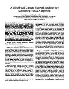
Fig. 1. This is an illustrative example of a scenario consisting of two cameras with their overlapping fields of view. Each field of view is depicted and numbered respectively. Two paths in different directions are also depicted demonstrating the generation of IN/OUT events.

In Figure 1 are depicted two cameras and theirs fields of view. The IN/OUT events are represented as well. Note that depending on the direction of the agent movement, the IN/OUT events may be registered in different zones. With reference to the Figure 1, the procedure of the Direct Voting Method (DVM), for collecting tentative pairs of IN/OUT events, is described. Supposing a single person traveling from the left to the right, and going step by step, the algorithm firstly registers the IN1 event and then the IN2. These two events are paired and it is generated the route IN1-IN2. The algorithm will vote it on group G ,, . Using the same procedure, the following routes are generated as well, IN2-OUT1, OUT1-OUT2. The correspondent votes are on the following groups: G ,, , G ,, , respectively. These routes can be named as valid routes because they infer the real relation of the cameras in study. 2.2 Area Voting Method The Area Voting Method (AVM) tries to pair an event with the closest events in time, in order to find valid routes as much as possible. The AVM follows a sliding window design. This sliding window has a predefined length in terms of number of events, let's say N. In this method, an event is paired with the others N events within the window. After this process, the window is shifted. The older event is removed and a new one is added, that should be the consecutive event of the most recent within the window. Then, all the process is repeated again. This method induces an increase of the probability of getting valid routes, in situations of higher disorder. However, it is computationally demanding, compared with the DVM. Let's introduce a hypothetical sequence of events registered from 5 cameras: IN1-OUT4-OUT3-IN2-OUT1-IN3-IN5OUT2-IN4-OUT1. The AVM technique will pair the first event with the second and vote on the correspondent group; will pair the first with the third and vote; will pair the first with the fourth and will repeat this process until the last event within the

sliding window. Next iteration, the second event is paired with the others events in the same way as explained for the first event. This process is repeated for all the events. 2.3 Entropy Analysis Since we tend to develop an automatic system able to estimate the topological relation of a network and perform it without Human intervention, is needed a process to estimate which voting method is the fitter for different situations during the events' registration. The entropy indicates the disorder of a system and it is a measure of the amount of information [15], and particularly in this study, it will inform about the probability of registering valid routes. It is possible to estimate the entropy of the system by analyzing the number of events per camera in a time frame. This means, from a starting period t0 to t1 a set of events are registered. Then, the following formula may be applied: Ω

=−

ln ( )

(2)

From the equation (2) the summation is over the total number of cameras, defining each one, a state i that the system can be in. The Pi are the probabilities for the system to be in these states, this means, the probability of an event be registered in the camera i. It is assumed in this work that the probability distribution over the set of cameras is a uniform distribution. Then, Pi is given by: 1 (3) Ω With the number of people going across the network increasing, the rate of generation of events increases as well. Consequently, the absolute level of entropy follows the same trend. Considering the possibility to predict situations where the disorder of the registered events is substantial, using the analysis's entropy, the objective is to anticipate these cases and choose automatically, which voting method is fitter to be used. =

2.4 Filters In this chapter will be presented some tools to detect which groups and routes may be considered as invalid. The first one is based on the type of routes that each group contains. Using the types of routes presented in the work [4], groups that do not match with any of those types, are eliminated. After the previous filter, in each group it is applied a vector quantization technique, LBG [14], to remove possible false routes. The LBG algorithm allows filtering the groups voted least, considering them false routes, and thus removing them from the following steps of the method. Finally, the smaller groups have a lower probability of being valid and they can be discarded.

From the remaining groups, a semantic analysis is performed to classify certain types of groups that are unique to indicate a relationship between cameras. Groups Classification. As already explained, each group contains all the routes of the same type and with the same characteristics. Thus, if a group does not fit with any of the 5 types presented in [4], it is constituted only by invalid routes, so it can be deleted. After this process, remain only the candidates to be valid groups and the next filters to be presented will try to remove potential invalid routes and groups. Filtering False Routes. For each registered event, we save its coordinates on the image, the ID of the respective camera, the time of its acquisition and if it is an IN or OUT event. Before executing the LBG algorithm, every route in each set is mapped into a 5D space, using the following vector notation: =(

,

,

,

, )

(4)

This notation comprises the image coordinates of the beginning and end points and the transit time between them. After that, the norm of the difference between each vector and the code-vector is calculated. The norm of each vector is then compared with the mean and the standard deviation of all the norms, as is demonstrated in the following equation. μ − ×

≤∥

∥≤ μ + ×

(5)

In the equation (5) μv and σv denote the mean and the standard deviation of all the norms, respectively and c is a constant that defines the range of acceptance. Typically, this constant varies within the interval [1–2] and with it, good results are obtained. After the comparison, the norm of the vectors that do not respect the equation (5) are considered as invalids and are eliminated. Hopefully, since in the false sets the routes are more spread, is probable that this filter could eliminate more routes than in the valid sets. Cleaning False Groups. At the first stage, the number of routes on each set is calculated and afterward the following restriction, represented by the equation (6) is applied. ≥μ − ×

(6)

Where ni is the number of routes in the set i, μb and σb denote the mean and the standard deviation of the numbers of the routes in the sets, respectively. The constant c establishes the range of acceptability for the sets. Typically, this constant assumes the value 1 and with it, good results are obtained. For each set, if the number of routes that constitute a set do not satisfy the condition imposed by the equation (6), this set is considered as a false set, and it is removed. After the capture of a certain number of events and after the LBG algorithm to be performed through all the sets, it is expected that the number of routes within the valid sets is much higher that the invalid sets. 2.5 Steps for the Topological Map Algorithm In this section is presented all the steps by the algorithm to estimate the topology of the network, in the correct order.

1.

2.

3.

4.

5. 6. 7. 8. 9.

Capture and Entropy. During a short period a group of events should be captured to perform the entropy's analysis. The experiments were made with 1 minute of time, concerning the scenario used. Indeed, this slice of time to be used on the entropy's analysis should be adjusted for different situations. Analysis Entropy's and Votes. Let's assume that during 1 minute are captured 50 events and then is performed the entropy's analysis. With this analysis and with the predefined levels, the best method is chosen to be executed. Furthermore, the 50 events are paired and voted using that method. Vote up to a Limit. The previous two steps are executed until a threshold is reached. Let's define this threshold as 500 votes made. When this threshold is reached, the filters are applied to the sets, as will be explained in the following steps. Remove Sets without a type associated. After the conclusion of the previous stage, the types of routes of all the sets are compared with the five types defined previously. In the cases that a match is not found, the sets are removed. Sum the reversed Sets. With the remaining sets from the previous step, the correspondent reversed sets are found and added together. Execution of the LBG Algorithm. In this stage, the LBG algorithm is performed. Consequently, the sets will contain less aggregated routes. Remove Invalid Sets. After the application of the LBG algorithm, the sets that do not have enough votes are eliminated. Semantic Information. Perform a semantic analysis. Incoherence in the obtained sets should be controlled. Topological Map Extraction. The topological information can be extracted from the sets that survived to the filters.

3 Experimental Results The events that are captured in real scenarios can be modeled as a stochastic process. This can be done because there is always a probability associated in determining which event is the next and the future events are independent of the past events, they depend only upon the present event. Using a matrix with all the transition probabilities is possible to model the people traveling within the network and passing through determined places. The Figure 2 depicts, in a general way, the matrix with the transition probabilities. Each camera has two types of events, so each camera will generate two possible stages in the matrix of the transition probabilities. One property of this matrix is that in each line the sum of the probabilities is always equal to 1, because all the possible , events are being considering in the matrix. Each value , represents the probability of being detected an event Ei in the camera i and the next event happens in the camera j with the type Ej. These probabilities should be consistent with the design and the ordering of the cameras, this means, the probability of the next event should be adequate to what is the present event.

Fig. 2. This figure shows the matrix of transition probabilities between possible states.

With this matrix constructed, the process will jump between the lines, triggering events. The generated events are captured and the algorithm to estimate the topology is executed as explained before. This process runs until the user stops the execution. The matrix presented in Figure 3 models an experimental scenario illustrated in Figure 6. As is possible to conclude, the probabilities in this matrix vary with the proximity of the cameras and with the paths, which in this case are the corridors that connects these cameras. The other remaining distribution of probabilities over the other possible cases has the objective to model the situations where some captured routes are not valid, generating then false relations. We conducted several simulations to confirm the robustness of the proposed method. With the simulations was possible to stress the system and test our method in harder situations. Analysing the Figure 3 and Figure 6, the camera 1 and camera 2 have their fields of view overlapping; the camera 3 and 4 have their fields of view overlapping as well and finally, the camera 5 doesn't share its field of view with any camera. The results obtained with our method, should indicate this configuration and the same relation of the cameras.

Fig. 3. Matrix with the transition probabilities used in the simulations.

As is possible to conclude analyzing the Figure 3, the probability of the generation of valid routes is situated below or equal than 30%. This value demonstrates how much chaotic can be the system to be modulated to achieve good estimations.

The following figures depict the graph obtained, in different steps, during the execution of our method. The arcs in the graphs indicate that between those nodes there is a route connecting them. Moreover, if an arc has an arrow, this means that there is an overlapping area. Before performing any filter, all groups are available, as is illustrated in the Figure 4. However, the Figure 4 presents some routes that are invalid, represented as the arrows pointed for the same node. These arrows are indicating that there is an overlapping area with itself camera, and since this information is not meaningful for the objective of the topological calibration, they can be removed. Applying all the steps of the algorithm, the graph will be updated as the results of each step are obtained and introduced in the following steps. The final estimate of the topological calibration is represented in the Figure 5. Analysing this graph, the results obtained with our algorithm are correct when compared with the plant of the Figure 6. All topological relations between the cameras are disposed and represented correctly. In this case, our method achieved 100% of inferring topological relationships.

Fig. 4. Graph with all the groups without performing any filter.

Fig. 5. Graph with all the groups that have passed through the filters and all the steps of the algorithm.

Fig. 6. A plant picturing the scenario to be considered and it reveals the relation between the cameras.

4 Conclusion In this paper we have presented an overview of related works in building topological map of sensors which may or not contain overlapping areas. We have presented a solution for the problem of relating cameras when their fields of view are overlapping including the scenarios where a set of cameras is sparse over the space. For these cases, the current state of the art related with this subject revealed to be insufficient and with some flaws. In order to test the proposed method, simulations were performed to conclude about its robustness, reliability and validity. The proposed method revealed to be faster to converge, it can work in an on-line mode and it does not need any prior knowledge about the network of cameras. The results obtained are positive and adequate for the requirements initially outlined. Future work should be carried out to develop a method where it might contain the identification of the agents that are traveling within the network. This will be remove the dependency of time and introduce a more reliable relation which is the creation of routes composed by events generated by the same agent.

References 1. Makris, D., Ellis, T. J. and Black, J.: Bridging the gaps between cameras. In IEEE Conference on Computer Vision and Pattern Recognition, Washington DC, June (2004) 2. Marinakis, D. and Dudek, G.: A practical algorithm for network topology inference. In IEEE International Conference on Robotics and Automation, Orlando, Florida, May (2006)

3. Marinakis, D., Dudek, G., and Fleet, D.: Learning sensor network topology through Monte Carlo expectation maximization. In IEEE International Conference on Robotics and Automation, Spain, April (2005) 4. Ukita, N.: Probabilistic-topological calibration of widely distributed camera networks. Machine Vision and Applications, pp. 249-260. May (2007) 5. Ihler, A. T., Fisher III, J. W., Moses, R. L., and Willsky, A. S.: Nonparametric belief propagation for self-calibration in sensor networks. IEEE Journal of Selected Areas in Communication, pp. 809-819. April (2005) 6. Paskin, M. A., Guestrin, C. E., and McFadden, J.: A robust architecture for inference in sensor networks. In Proceedings of the Fourth International Symposium on Information Processing in Sensor Networks IPSN-05, (2005) 7. Dantu, K. and Sukhatme, G. S.: Rethinking data-fusion based services in sensor networks. In The Third IEEE Workshop on Embedded Networked Sensors, (2006) 8. Wang, H., Elson, J., Girod, L., Estrin, D., and Yao, K.: Target classification and localization in a habitat monitoring application. In Proceedings of the IEEE International Conference on Acoustics, Speech, and Signal Processing, pp. 214-226. (2003) 9. Songhwai Oh, M. M., Chen, P., and Sastry, S.: Instrumenting wireless sensor networks for real-time surveillance. In Proceedings of the International Conference on Robotics and Automation, May (2006) 10.Pasula, H., Russell, S., Ostland, M., and Ritov, Y.: Tracking many objects with many sensors. In International Joint Conference on Artificial Intelligence, Stockholm, (1999) 11.Rekleitis, I., Meger, D., and Dudek, G.: Simultaneous planning localization, and mapping in a camera sensor network. Robotics and Autonomous Systems Journal, special issue on Planning and Uncertainty in Robotics, (2005) 12.Djugash, J., Kantor, G., Singh, S., and Zhang, W.: Range-only slam for robots operating cooperatively with sensor networks. In Proceedings of the International Conference on Robotics and Automation, May (2006) 13.Lee, L., Romano, R. and Stein, G.: Monitoring Activities from Multiple Video Streams: Establishing a Common Coordinate Frame. IEEE Transactions on Pattern Analysis and Machine Intelligence, vol. 22, no. 8, pp. 758-767. August (2000) 14.Linde, Y., Buzo, A., Gray, R. M.: An algorithm for vector quantizer design. IEEE Transaction on Communications, pp. 84-95. (1980) 15.Haynie, Donald, T.: Biological Thermodynamics. Cambridge University Press. ISBN 0-52179165-0. (2001)