Operating Cost Aware Scheduling Model for Distributed Servers Based on Global Power Pricing Policies Sudha Mani
Shrisha Rao
International Institute of Information Technology Bangalore Bangalore,India
International Institute of Information Technology Bangalore Bangalore,India
[email protected]
[email protected]
ABSTRACT
1. INTRODUCTION
Reducing the power consumption and operational cost of IT servers is of great concern today. With the growth of the Internet and online services, the number of data centers is increasing day by day. Servers for many cloud applications and other large providers are spread globally. Energy costs across the globe vary dynamically. Servers operate at varied energy costs based on their location and time of use. The load of a server varies based on its geographical location and the time of operation. This paper focuses on exploiting the dynamic nature of electrical power pricing, so that a cost saving is obtained by geo-location of requests to servers operating at lower costs at particular times. There exist patterns of load that are similar for different types of servers. Scheduling decisions are made considering both loads and operating costs of the servers into account, i.e., requests are scheduled to run on servers operating at low cost that also have low expected load. In order to meet the business requirements of an application, scheduling decisions for requests that have stringent SLA considerations or high server affinity, are made by assigning high priority for these requests. Geo-location of requests is done for low priority requests.
The motivation for this paper is based on the growing importance of energy/power consumption of servers in data centers, i.e., the electricity cost incurred in order to operate them 24 × 7 and also to provide extensive cooling systems to keep their operating temperatures within thermal stability limits. Large data centers consume several megawatts of power which amounts to billions of dollars spent on energy costs. In addition to the cost of powering these servers, we also need to include the cost of deploying cooling systems (which in turn consume power) to ensure stable operation [5]. An analysis of Facebook’s spending with data centers indicates that the company paid about $50 million to lease data center space in 2010, compared to about $20 million in 2009 [1], a large increase that suggests a corresponding increase in the energy costs associated with their data centers. Servers handling client requests are geographically distributed and the market price of energy varies based on region and time. Energy costs vary every hour at various places. Therefore, servers providing the same service may operate at different costs based on their location and times of operation. Client requests can be scheduled to servers that operate at lower costs at particular points of time. We therefore propose that the load should be geo-located in such a way that servers operating at lower cost are preferred, and among them, those at a lower load. For data centers, it is important to reduce the cost of operation while meeting the required Service Level Agreement (SLA) in terms of response times and other quality metrics. Load balancing is needed at these centers to provide the right resources to the right service being hosted, at the right time, so that their operational cost is reduced while still meeting any performance based SLAs [5]. While rescheduling requests to a different server operating at lower cost, the priority of the request based on server affinity is considered. The approach presented in this paper focuses on distributing the workload among different geo-distributed data centers when required, to reduce the operating cost by considering the energy cost and load factor of the servers. As the servers are globally distributed, the time difference between different data centers, which determines their load, is made use of while scheduling requests. Therefore, servers running the same application can receive different numbers of requests, i.e., operate at varying loads based on time. In such cases, servers operating at low cost with low workload can be utilised the most. Also, there might be servers that are not utilised to their full capacity. The new jobs which require additional number of
Categories and Subject Descriptors C.2.4 [Distributed Systems]: Distributed applications; C.2.5 [Local and Wide-Area Networks]: Internet; C.4 [Performance of Systems]: Design studies; D.4.8 [Performance]: Simulation; H.3.4 [Systems and Software]: Distributed systems
General Terms Algorithms, Economics, Management, Performance
Keywords distributed servers, scheduling, operating cost, energy cost
Permission to make digital or hard copies of all or part of this work for personal or classroom use is granted without fee provided that copies are not made or distributed for profit or commercial advantage and that copies bear this notice and the full citation on the first page. To copy otherwise, to republish, to post on servers or to redistribute to lists, requires prior specific permission and/or a fee. COMPUTE’11, Mar 25-26 2011, Bangalore, India Copyright 2011 ACM 978-1-4503-0750-5/11/03 ...$10.00.
servers to operate in a particular group, when routed can fit into the capacity of the servers operating at low load, without requiring additional servers. This in turn would lead to reduction in the total number of servers required for an application which also adds up to the reduction in operating cost. In our case study we found 30 % reduction in the number of servers required (Fig. 7). The customized Global Distributed Dynamic Load Balancing (GDDLB) [20] algorithm which takes energy cost and loads of servers also into account is used for this approach. Simulation results using data about Facebook servers shows that 16.5% of cost is saved by considering only the energy cost factor while scheduling. By taking the time of operation also into account which determines the load of the server, 18.5% of cost saving is obtained. The rest of the paper is organised as follows. Section 2 discusses the related work. Section 3 describes the proposed system model and load balancing strategy. Section 4 discusses the scheduling algorithm used. Section 5 discusses the cost saving calculations. Section 6 dicusses the case studies used to simulate the approach proposed. Section 7 gives some concluding remarks and discusses possible future work.
2.
RELATED WORK
In previous works, efforts have been made to optimize energy first, with a slight degradation in response time. By optimizing the energy consumption, the operating cost is also reduced. There are approaches to reduce the power consumption within data centers by turning off or hibernating idle servers or by using dynamic voltage/frequency scaling technologies [5, 7]. Energy management for server clusters found in data/hosting centers has been addressed in previous studies [12, 10, 8, 9]. Some early studies [10, 14] show that energy management and cost management can be related by developing techniques for shutting down servers that are not in use or have low load (by offloading their duties to other servers). Studies [9, 18] have looked at optimizing the power consumed by the CPU, by monitoring evolving load and performance metrics to dynamically modulate CPU frequencies. There are schemes that consider server shutdowns and/or allow dynamic voltage scaling and they also focus on energy management of just one server and try to meet SLAs imposed by the applications, and the solutions also incorporate the cost of rebooting servers. Chen, et al. [5] present a formalism for the power and cost management problem, and propose three new online solution strategies based on steady state queuing analysis, feedback control theory, and a hybrid mechanism, borrowing ideas from these two. Using real web server traces, they show that these solutions are adaptive to workload behavior when performing server provisioning and speed control, thus minimizing operational costs while meeting the SLAs. Earlier works [4, 19, 21, 16, 15, 17] have discussed the dynamic scheduling algorithms that take various parameters into account while scheduling requests in a distributed environment.
3.
SYSTEM MODEL AND LOAD BALANCING STRATEGY
A distributed client server architecture is used for implementing the system model (Fig. 1). Assumptions made in the system model are as follows: 1. The tasks are atomic, i.e., cannot be subdivided into
Figure 1: Distributed Client Server Architecture
smaller tasks that can be scheduled on different servers for execution. 2. There is no task migration. Scheduling is done only for new incoming tasks. 3. There are two types of requests in the system, based on their server affinity. They are prioritized accordingly. The server-specific requests have high priority and other requests that are not server-specific are assigned low priority. 4. Each server has the same capacity to service requests or jobs that are more or less uniform in size.
Group-based Approach The distributed servers are divided into various groups based on operating cost, i.e., based on the energy costs at the regions where the servers operate. All servers that operate at the same energy cost at a given instant of time form a group. In case of servers in data centers, one or more data centers can be part of a group. Each group has a master server. Master servers of all groups are connected. The master of a group has the following tasks: • It broadcasts its operating cost information to all its fellow master servers. • Based on the historical pattern of the priority requests, it calculates the available capacity of its group and broadcasts the same. • It geo-locates the client requests to a server based on minimum operating cost and minimum load. • It schedules the high priority requests to the server requested by the client and does not route it further. • It runs a modified kNN algorithm [11] on the historical data of load to predict the load at a given time.
Dynamic Load Balancing Strategy Distribution of work among the servers has to be done dynamically at runtime based on the varying operating costs at different regions and at different times. The energy cost varies every hour in different regions. The number of incoming requests to servers also varies dynamically. Therefore, a dynamic load balancing algorithm is used. The load balancing algorithm employed depends on three major parameters [13]. These parameters define: 1. Who makes the load balancing decision? (Is it the receiver or the sender?) 2. What information is used to make the load balancing decision? 3. Where is the load balancing decision made? In our model, the master server makes the load balancing decision by making use of the energy cost information of the distributed servers.
Receiver-Initiated Strategy The question of who makes the load balancing decision is answered based on whether a sender-initiated or receiverinitiated policy is employed. In receiver-initiated policies, nodes operating at lower cost look for nodes operating at high cost from which jobs can be received [13]. At high system loads, receiver-initiated policies perform better [13]. For our approach, we choose a receiver-initiated policy. The master server of the receiver group sends information about its current operating cost and available capacity to all its fellow masters. It sends a stop message to all its neighbors, if it has no available capacity to service additional requests.
4. GDDLB APPROACH AND SCHEDULING ALGORITHM In our system model, a group based approach is employed, as mentioned earlier. Servers operating at the same cost at a particular instant of time form a group. The energy cost varies every hour in reality. Therefore, the group is reconfigured every one hour based on the energy cost. In our model, a receiver-initiated strategy is applied. The receiver at a particular instant of time is the group that operates at lower cost than other groups and that has capacity to service new requests. Such a receiver advertises its available capacity to service requests to its neighbors, i.e., the master server of the receiver group advertises the available capacity of its group, to the fellow master servers. The capacity of a server is defined in terms of the number of requests that can be serviced by the server per hour. Hence the receiver group is identified based on the operating cost of each group and its load data. The masters of the groups exchange the operating cost detail among them. For every time interval when the operating cost changes, cost details are exchanged among the master servers and the groups are reconfigured. Master servers exchange an operating cost vector of size equal to the number of groups at a particular time. The master updates its operating cost in the vector and sends it to its neighbors. The master server of each group maintains the historical data of the load of its group. It runs a modified kNN algorithm [11] on the historical data to predict the load at a given time. Let, 1. G be the set of total number of groups 2. i be the index used to refer a group, where 0 < i ≤| G | 3. ni be the number of servers required by group i at particular time instant to service its regular load
Global Strategy
4. Ni be the total number of servers in group i
In the global schemes, the load balancing decision is made using global knowledge. A dedicated load balancer uses the performance profiles of all available servers. All the processors take part in the synchronization, and send their performance profiles to the load balancer. For global schemes, balanced load convergence is faster since data of all the servers are considered at the same time (By contrast, in the local schemes, the work re-distribution is not optimal, resulting in slower convergence). However, this requires additional communication and synchronization between the various workstations [13].
5. T be the time at which the energy cost varies (one hour)
Distributed Strategy The load balancer is replicated in the representative master server of each group. A distributed strategy provides a scalable solution. Therefore the load balancing algorithm chosen for our purpose is a Global Distributed Dynamic Load Balancing (GDDLB) algorithm [15]. Zaki et al. [20] discuss the customized load balancing algorithm which is essential for good performance. Their work presents a hybrid compile-time and run-time modeling and decision process that selects the best scheduling scheme for a particular system. This algorithm with additional parameter of operating cost is used for GDDLB based on operating cost and load at which it operates.
6. Op cost be operation cost vector hC0 , C1 , . . . , CG i, where Ci is the operating cost(energy cost) of group i 7. Mi be the master server of group i 8. Local op costi be the copy of the Op cost in master server Mi of group i 9. αt,i be the total capacity of group i to service requests 10. αp,i be the predicted load of group i at a particular time using modified kNN algorithm 11. αa be the available capacity vector hα0 , α1 , . . . , αG i, where αi is the available capacity of group i 12. task priority(k) be the priority assigned to the task k based on server affinity 13. Gmin (t) be set of groups operating at low cost at time t, where Gmin (t) ⊆ G 14. Aβ be the available capacity of group β, where group β has the maximum available capacity in the set of groups operating at low cost, β ∈ Gmin (t)
The messages exchanged between master servers of each group are as follows: Let, • Inf ohOp costi be the message used by the master server of each group, to exchange the operating cost of its group with the others, at every time interval when the operating cost varies, i.e., for every t. • Readyhαa i be the message sent by the master server of the receiver group to advertise its available capacity to other groups operating at high cost.
1 3 2 4 5 6 7 8
• Stophi be the message sent by the master server of the receiver group to its neighboring master servers, to stop sending requests when it has no available capacity.
At receiver side: for every T do Send Inf ohOp costi end while true do if αa [i] == 0 then Send Stophi end else Send Readyhαa i end end At Sender Side :
On receiving Inf ohOp costi from Mj Set Local op costi = Op cost On receiving Stophi from Mj Set αa [j] = 0 Set Local op costi [j] = ∞ On receiving Readyhαa i from Mj Set αa [j] in Mi = αa [j] from Mj Set Local op costi [j] = Op cost[j] 16 Algorithm 1: Operating cost and available capacity advertisement in master server Mi of group i 9
• T askhki be the message sent by the master server of a group to route task k to the other groups The available capacity of a group i at a particular instant of time, is the difference between the total capacity of the group and the capacity required by the group to service its regular load at that instant. The available capacity of group i can be calculated using the equation below. αi = αt,i − αp,i
(1)
When a master server of a group i receives Stophi message from a group j, it sets the available capacity value of that group to zero in its available capacity vector, i.e., αa [j] = 0 and sets the operating cost information of that group in its local cost vector as infinity, i.e., Local op costi [j] = ∞. Hence this group will not be considered for scheduling by the master server. When a receiver group is ready to service requests it sends a Readyhαa i message with its available capacity information. A master server of group i on receiving ready message from a receiver, updates the available capacity of that group j in its available capacity vector to the capacity information in the received message, i.e., αa [j] in Mi = αa [j] from Mj and updates the operating cost of that group in local copy of cost vector, from the Op cost vector received at the last group configuration time(t), i.e., Local op costi [j] = Op cost[j]. Scheduling algorithm is run in all the master servers of each group. The incoming tasks/jobs/requests of a group is assigned priority based on the server affinity as mentioned earlier. The master server schedules the high priority tasks to the requested group. It routes the low priority requests to servers operating at low cost and also have low load, according to our proposed approach. The set of server groups operating at low cost is identified by the master server from the local operation cost vector. Among those servers, the servers having low load is identified using the available capacity vector. The functions used in the scheduling algorithm are as follows. • Schedule T ask() is the function that schedules the task to a server in a group • Route() is the function that schedules the low priority based requests • M in(Local op costi ) returns a set of groups operating at low cost using the cost information of groups from Local op costi vector
10 11 12 13 14 15
for every task k in Mi do if task priority(k) == HIGH then Schedule T ask() to group i end else 4 Route() end end Algorithm 2: Operating Cost Aware Scheduling for Mi
1 2 3
• M ax Avail(Gmin (t), αa ) returns the maximum available capacity of server from the set Gmin (t) using the available capacity vector αa Algorithm 2 explains the scheduling approach used in this model. If the task priority(k), i.e., priority of the task k is high then it schedules it to the same group i. If the priority is low it calls the Route() function which does the scheduling for the low priority requests. Algorithm 3 explains the Route() function. Gmin (t) is the set of server groups operating at low cost. If the group i which received the task k is in the minimum set Gmin (t), then task is scheduled to group i that received the task initially. Otherwise, the group with maximum capacity (or the least traffic) is chosen using M ax Avail(Gmin (t), αa ) function. The task is sent to the chosen group β. If the chosen group has no available capacity, then Route() is called recursively, so that a different receiver group can be found.
5. COST SAVING CALCULATION Let us assume that group i is the sender and group j as the receiver chosen by the master server Mi . ni is the number of servers required for servicing requests in group i at time t1 and nj is the number of servers required for servicing requests at time t2 in group j. Ni and Nj are the total numbers of servers in groups i and j respectively. Ci is the
1 2 3 4 5 6 7 8 9
Gmin (t) = M in(Local op costi ) if i ∈ Gmin (t) then Schedule T ask() end else Aβ = M ax Avail(Gmin (t), αa ) if Aβ 6= 0 then Send T askhki to group β end else Route() end end Algorithm 3: Code for Route()
cost of operating a server in group i, i.e., Ci = Op cost[i], and Cj = Op cost[j] is the cost of operating a server in group j. Let each server consume energy E. Energy consumed by group i, Ei is given by, Ei = ni × E
(2)
Energy consumed by group j, Ej is given by, Ej = nj × E
(3)
When the proposed solution is not applied, there is no rescheduling of the requests based on energy cost. Therefore, total cost of operation across all groups, Ctotal is given by, Ctotal = (ni Ci + nj Cj )
(4)
As group j is the receiver chosen, operating cost of group j is lower than that of group i, i.e., Ci > Cj . By implementing the proposed solution, requests are routed to servers in a group operating at lower cost until it is used to its maximum available capacity. Therefore, group j operating at lower cost will be utilized maximum, i.e., Nj servers will be utilized. (Nj − nj ) servers are available in group j to service jobs from other groups. Requests corresponding to (Nj −nj ) servers in the group i are re routed to group j. ′ If ni ≤ (Nj − nj ), total cost of operation, Ctotal is given by, ′ Ctotal = (ni + nj )Cj
is given by,
= [ni − (Nj − nj )]Ci + Nj Cj
(6)
If ni > (Nj − nj ), total cost of operation, ′ Ctotal
(5) ′ Ctotal
Total cost saving when ni ≤ (Nj − nj ) is given by, CostSaving (∆C) = (Ci − Cj ) × ni
∆Cj = (Ci − Cx )(Nx − nj )
(9)
Total cost saving when requests are cheduled to group k (7)
Total cost saving when ni > (Nj − nj ), CostSaving (∆C) = (Ci − Cj ) × (Nj − nj )
at energy cost 13 cents/kWh and 8 cents/kWh respectively. Total cost of operation without considering the solution at t1 = operating cost of group i at t1 + operating cost of group j at t1 = (50 × E × 13) + (50 × E × 8) = 1050E Total cost of operation considering the solution at t1 = operating cost of group i at t1 + operating cost of group j at t1 = (0 × E × 13) + (100 × E × 8) = 800E Total cost of operation without considering the solution at t2 = operating cost of group i at t2 + operating cost of group j at t2 = (80 × E × 13) + (80 × E × 8) = 1680E Total cost of operation considering the solution at t2 = operating cost of group i at t2 + operating cost of group j at t2 = (60 × E × 13) + (100 × E × 8) = 1580E Therefore, from the above calculation, it is observed that operating cost is reduced by implementing the proposed solution. When considering the time zone difference at different places, the number of servers required at an instant of time will vary as the number of requests will vary as observed from the traffic pattern as shown in Fig. 3. Therefore if requests are geo-located to the group operating in a time zone such that it operates at lower load and less cost, it results in greater cost saving. Let ni be the number of servers required for servicing requests in group i at time t1 and nj , the number servers required for servicing requests at time t2 in group j. At t2 group k has less traffic compared to group j and requires nk servers for servicing requests. Therefore nj > nk . Let Ni be the total number of the servers in group i and let us assume the total number of servers in group j and group k are equal. Total number of servers in group j = Total number of servers in group k = Nx Ci = Op cost[i] is the cost of operating a server in group i and operating cost of group j = operating cost of group k = Cx = Op cost[j] = Op cost[k]. If ni ≤ (Nx − nj ) and ni ≤ (Nx − nk ), then re routing requests to either one of them will result in same amount of cost saving. If ni > (Nx − nj ) and ni > (Nx − nk ), then from Equation 8, Total cost saving when requests are scheduled to group j
(8)
For example, consider group i and group j to have the total capacity Ni = Nj = 100 and E be the energy consumed by each server. Let 50 servers be required by both the groups at time t1 and 80 servers at time t2 . At time t1 , group j has 50 servers available to service requests from other groups. Therefore, requests corresponding to 50 servers in group i are routed to group j. By implementing our solution, 100 servers in group j will operate and 0 servers in group i will operate at time t1 . At time t2 , 20 servers in group j are available. Therefore, 60 servers of group i and 100 servers of group j will operate at t2 . Let group i and group j operate
∆Ck = (Ci − Cx )(Nx − nk )
(10)
Since nj > nk , ∆Ck > ∆Cj . Therefore, considering the time zone difference into account, percentage increase in cost saving is ((nj − nk )/(Nx − nj )) × 100. For example, consider group i, group j and group k to have the total capacity of 100 servers each and E be the energy consumed by each server. Let us assume that group i and group j operate at the same load, i.e., belongs to the same time zone and group k belongs to a time zone which operates at low load at time t. Let 20 servers be required by both the groups j and k at time t and 80 servers by group i at time t. By implementing our solution, 100 servers in group k will operate and 0 servers in group i will operate at time t. Let group i and group j operate at energy cost 13 cents/kWh and group k operates at 8 cents/kWh .
Figure 3: Web Client Traffic for a Day on an International Link
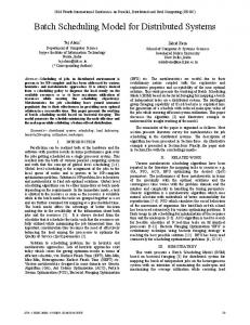
Figure 2: Geographical Distribution of Facebook Servers
Total cost of operation without considering the solution at t= operating cost of group i at t + operating cost of group j at t + operating cost of group k at t = (80 x E x 13) + (20 x E x 13) + (20 x E x 8) = 1460E Total cost of operation considering the solution at t= operating cost of group i at t + operating cost of group j at t + operating cost of group k at t = (0 x E x 13) + (20 x E x 13) + (100 x E x 8) = 1060E
6.
CASE STUDIES
For studying the proposed approach, Facebook servers are considered. Facebook at present has servers only in the United States of America. It currently operates out of nine data centers in the United States: six on the west coast and three on the east coast of the USA [1]. Their six data centers are in California (CA) and three data centers are in Virginia (VA) State (Fig. 2). The energy cost of California is higher compared to that at Virginia. The average energy cost of California is 13.97 cents per kWh and that of Virginia is 7.72 cents per kWh for commercial purposes [3]. Assumptions made for simulation: • The data centers in Virginia and California have 7000 servers each. • Each server can service 50 requests per minute. Our calculation is done in two steps.
Case 1 First, we analyze the cost saving by considering only the energy cost factor. For this, we assume that there exists a similar pattern of load for all the data centers over a day. We assume that the Internet traffic follows the pattern as shown in Fig. 3. It shows the real time web client traffic for a day on an international link. Average power usage of a server is 454.39 W [6]. For case 1, we require equal number
Figure 4: Cost Curve of Servers Without the Solution
of servers at different data centers to service the requests, as we have assumed same load pattern and time of operation for all the servers considered. Based on the number of requests, number of servers required can be calculated. Based on the assumption made, Number of servers required = (Total number of requests at a particular time / 50) Figure 5 shows the cost curve of servers at California (CA) and Virginia (VA) considering only the cost factor.
Case 2 In the second case, we analyze the cost saving obtained by considering energy cost factor and load factor into account. As mentioned earlier, the load of a server is dependent on the time of operation. If there is a time difference between servers operating at different time zones, then there will be variation in the load at which they operate. This variation in load leads to varying numbers of servers required at every instant of time. Therefore, there will be unequal number of servers required at every instant unlike the case 1 considered above. Using Eq. 5 and Eq. 6 the total cost of operation considering the cost factor and load factor can be calculated. Figure 6 shows the cost curve of servers at California (CA) and Virginia (VA) based on the cost factor and load factor.
Simulation Results Using Eq. 2 and Eq. 3 the energy consumed by the servers is calculated without implementing the proposed approach. From the energy consumption details, operating cost of servers at California and Virginia can be obtained. Figure 4 shows
Cost Saving Results Factors
Operating Cost/day
Cost Saving
Energy Cost Energy Cost & Load
$1.14 million $0.95 million $0.932 million
0% 16.5% 18.5%
Table 1: Cost Saving Calculation
Figure 6: Cost Curve of Servers on Scheduling Requests Considering Energy Cost and Load Factor
Figure 5: Cost Curve of Servers on Scheduling Requests Considering Energy Cost only
the energy cost curve of servers in the two states without implementing the solution. It also assumes the servers at both states have the same load patterns. Using Eq. 4, Total cost of operation across two states is found as 1.14 million dollars/day as shown in table 1. In case 1, we consider only the cost factor into account. Virginia operates at lower cost compared to California. Therefore the servers at Virginia are utilized to the maximum. Using Eq. 5 and Eq. 6 the total cost of operation considering the cost factor is found as 0.95 million dollars/day as shown in Table 1. Cost saving obtained is calculated using the Eq. 7 is 16.5%. In case 2, we consider both the cost and load factor into account. California and Virginia has the time difference of 3 hours [2]. Total cost of operation across two states without solution is found as 1.13 million dollars/day. Load of the server is highly dependent on time. Hence, the cost aware scheduling taking the time difference into account leads to increase in cost saving. Load pattern of servers at the two states vary with respect to time of operation as shown in Fig 3. Using Eq. 5 and Eq. 6 the total cost of operation considering the cost factor and load factor is found as 0.932 million dollars/day. Cost saving calculated using the Eq. 7 is 18.5%. From Fig. 7 it can be observed that the total number of servers operating in CA is reduced, when the time difference is taken into consideration. Thus the operating cost is reduced by making maximum utilization of the servers in VA. The reduction in total number of servers also aids in reducing the power consumed by the data centers in total to a small extent. This is an additional advantage of this approach. Figure 8 shows the operating cost with and without implementing the solution.
Figure 7: Server Requirement Pattern for Facebook Servers
7. CONCLUSIONS AND FUTURE WORK Reducing the power consumption and operating cost of huge data centers is of great concern today. In this paper we address the problem of high electricity cost incurred to run distributed servers for various applications. We have proposed a solution that optimizes operating cost and also caters to the performance needs of the application, taking priority requests into consideration. The proposed solution shows potential in reducing the operating cost by using GDDLB algorithm. This algorithm takes the operating cost parameter and the time zone of location of servers into consideration. Our approach ensures that the servers operating at lower cost do not miss out on the regular traffic, by taking the historical pattern of traffic into consideration and calculating the available capacity based on it. The operating cost optimization based on global power pricing policy does not seem to be addressed in previous works. Scheduling of requests taking the energy cost of the operating servers into account is the novel idea proposed here. We demonstrate the efficacy of our solution by simulating the cost saving using real data. Simulation results on regular traffic at the organizational level showed a cost saving of 20% on average. This solution will be highly useful for those applications that have soft constraints with respect to SLAs. While re-scheduling the requests, the network cost associated with servicing requests are not considered. This will be considered as a part of the future work.
[10]
[11]
[12]
[13] Figure 8: Cost Saving Obtained With Solution
8.
[14]
REFERENCES
[1] Data Center Knowledge, 2010. http://www.datacenterknowledge.com/archives/. [2] timeanddate.com, 2010. http://www.timeanddate.com/worldclock. [3] U. S. Energy Information Administration, 2010. http://www.eia.doe.gov/electricity/epm/table5 6 b.html. [4] A. M. Alakeel. A guide to dynamic load balancing in distributed computer systems. IJCSNS International Journal of Computer Science and Network Security, 10(6), June 2010. [5] Y. Chen, A. Das, W. Qin, A. Sivasubramaniam, Q. Wang, and N. Gautam. Managing server energy and operational costs in hosting centers. ACM SIGMETRICS Performance Evaluation Review, 33(1):303–314, 2005. [6] R. Chheda, D. Shookowsky, S. Stefanovich, and J. Toscano. MSDN, 2010. http://msdn.microsoft.com/enus/library/dd393312.aspx. [7] S. Dangi, D. Karnam, C. Madhavan, S. Mani, and S. Rao. Self tuning energy-aware ensemble model for server clusters. In Annual International Conference on Green Information Technology (GREENIT 2010), Singapore, Oct. 2010. [8] E. Elnozahy, M. Kistler, and R. Rajamony. Energy-efficient server clusters. Power-Aware Computer Systems, pages 179–197, 2003. [9] M. Elnozahy, M. Kistler, and R. Rajamony. Energy conservation policies for web servers. In Proceedings of the 4th conference on USENIX Symposium on
[15]
[16]
[17]
[18]
[19]
[20]
[21]
Internet Technologies and Systems-Volume 4, page 8. USENIX Association, 2003. J.Chase and R.Doyle. Balance of power: Energy management for server clusters. In Proceedings of the 8th Workshop on Hot Topics in Operating Systems, May 2001. T. Kim, H. Kim, C. Oh, and B. Son. Traffic flow forecasting based on pattern recognition to overcome memoryless property. In Multimedia and Ubiquitous Engineering, 2007. MUE’07., pages 1181–1186. IEEE, 2007. C. Lefurgy, K. Rajamani, F. Rawson, W. Felter, M. Kistler, and T. Keller. Energy management for commercial servers. Computer, 36(12):39–48, 2003. S. Malik. Dynamic Load Balancing in a Network of Workstations. 95.515 Research Report, 19, 2000. E. Pinheiro, R. Bianchini, E. Carrera, and T. Heath. Load balancing and unbalancing for power and performance in cluster-based systems. In Workshop on Compilers and Operating Systems for Low Power, volume 180, pages 182–195. Citeseer, 2001. A. Piotrowski and S. Dandamudi. A comparative study of Load Sharing on Networks of Workstations. In Int. Conf. Parallel and Distributed Computing Systems, pages 458–465. Citeseer, 1997. R. Shah, B. Veeravalli, and M. Misra. On the design of adaptive and decentralized load balancing algorithms with load estimation for computational grid environments. IEEE Transactions on parallel and distributed systems, 18(12):1675–1686, 2007. S. Sharma, S. Singh, and M. Sharma. Performance Analysis of Load Balancing Algorithms. In Proceedings of world academy of science, engineering and technology, volume 28, pages 1307–6884, 2008. V. Sharma, A. Thomas, T. Abdelzaher, K. Skadron, and Z. Lu. Power-aware QoS management in web servers. In Real-Time Systems Symposium, 2003. RTSS 2003. 24th IEEE, pages 63–72. IEEE, 2005. Y. Wang and R. Morris. Load sharing in distributed systems. Computers, IEEE Transactions on, 100(3):204–217, 2006. M. Zaki, W. Li, and S. Parthasarathy. Customized dynamic load balancing for a network of workstations. In High Performance Distributed Computing, 1996., Proceedings of 5th IEEE International Symposium on, pages 282–291. IEEE, 2002. Z. Zeng and B. Veeravalli. Design and analysis of a non-preemptive decentralized load balancing algorithm for multi-class jobs in distributed networks. Computer Communications, 27(7):679–693, 2004.