cooling cost. Since processors consume a large percent- age of energy in computer systems, especially in embedded systems, much work has been done on ...
Proc. of the Int. Parallel and Distributed Processing Symposium, Apr. 2003
Energy Aware Scheduling for Distributed Real-Time Systems∗ Ramesh Mishra, Namrata Rastogi, Dakai Zhu Daniel Moss´e and Rami Melhem Computer Science Department University of Pittsburgh Pittsburgh, PA 15260 {ramesh,namrata,zdk,mosse,melhem}@cs.pitt.edu
Abstract Power management has become popular in mobile computing as well as in server farms. Although a lot of work has been done to manage the energy consumption on uniprocessor real-time systems, there is less work done on their multicomputer counterparts. For a set of real-time tasks with precedence constraints executing on a distributed system, we propose new static and dynamic power management schemes. Assuming a given static schedule generated from any list scheduling heuristic algorithm, our static power management scheme uses the static slack (if any) based on the degree of parallelism in the schedule. To consider the run-time behavior of tasks, an on-line dynamic power management technique is proposed to further explore the idle periods of processors. By comparing our static technique with the simple static power management, where the static slack is distributed to the schedule proportionally, we find that our static scheme can save an average of 10% more energy. When combined with dynamic schemes, our schemes significantly improve energy savings.
1 Introduction Energy aware computing has recently become popular not only for mobile computing systems to lengthen battery life but also in large systems consisting of multiple processing units to reduce energy consumption and associated cooling cost. Since processors consume a large percentage of energy in computer systems, especially in embedded systems, much work has been done on managing energy consumption for processors. Based on the dynamic voltage scaling (DVS) technique, energy management schemes in ∗ This work has been supported by the Defense Advanced Research Projects Agency through the PARTS project (Contract F33615-00-C1736).
uniprocessor real-time systems have been extensively explored. Fewer works, however, have focused on energy management for parallel and distributed real-time systems. For shared memory systems, we have recently proposed some power management schemes for real-time applications based on global scheduling techniques [27, 28]. In this paper, we address energy management for distributed real-time systems, where the communication time is significant and tasks may have precedence constraints. We start by taking a schedule that is generated from some scheduling discipline, such as list scheduling, and then apply two techniques to enhance the power management of the system. The mapping of tasks to processors and static scheduling algorithm used in this work is taken from [21]. First, we propose a new static power management scheme based on the degree of parallelism in the schedule. Then, to further explore the task’s run time behavior, we propose two dynamic techniques, greedy and gap-filling to use the processor idle periods to execute tasks at reduced speeds for more energy savings. Our algorithms manage slack that is dynamically created to slow down scheduled tasks as well as to change the order in which tasks were originally scheduled. The paper is organized in the following way. The related work is addressed in Section 2. The application, power and system models are described in Section 3. Static power management scheme is addressed in Section 4. Section 5 discusses the dynamic power management scheme and simulation results are shown and analyzed in Section 6. Finally Section 7 concludes this paper.
2 Related Work Many hardware and software techniques have been proposed to reduce the energy consumption of such systems, such as shutting down unused components and low energy circuit designs. With CMOS technology, processor’s power is dominated by dynamic power dissipation which is de-
termined by processor supply voltage and clock frequency [4, 6]. By reducing processor clock frequency and supply voltage, we can reduce energy consumption at the cost of performance of processors. Processors with the ability of dynamic voltage scaling (DVS) are currently commercially available [11, 10]. There is an interesting trade-off between the energy consumption and performance of processors, especially for real-time systems in which high performance is sometimes necessary in order to meet the timing constraints. For uniprocessor systems, Weiser et al. first discussed the problem of scheduling tasks to reduce the energy consumption of processors [23]. Yao et al. described an off-line scheduling algorithm for independent tasks running with variable speed, assuming worst-case execution time [25]. Based on dynamic voltage scaling (DVS) technique, Moss´e et al. proposed and analyzed several schemes to dynamically adjust processor speed with slack reclamation [18]. In [22], Shin et al. set the processor’s speed at branches according to the ratio of the longest path to the taken paths from the branch statement to the end of the program. Kumar et al. predict the execution time of tasks based on the statistics gathered about execution time of previous instances of the same task [13]. The best scheme is an adaptive one that takes an aggressive approach while providing safeguards that avoid violation of the application deadlines [2, 17]. When considering limited voltage/speed levels in uniprocessor systems, Chandrakasan et al. have shown that, for periodic tasks, a few voltage/speed levels are sufficient to achieve almost the same energy savings as infinite voltage/speed levels [5]. Pillai et al. also proposed a set of scheduling algorithms (static and dynamic) for periodic tasks based on EDF/RM scheduling policy [19]. AbouGhazaleh et al. have studied the effect of voltage/speed adjustment overhead on choosing the granularity of inserting power management points in a program [1]. For periodic task graphs and aperiodic tasks in distributed systems, with a given static schedule for periodic tasks and hard aperiodic tasks, Luo et al. proposed a static optimization algorithm by shifting the static schedule to redistribute the static slack according to the average slack ratio on each processor element [15]. They improved the static optimization by using critical path analysis and task execution order refinement to get the maximal static slow down factor for each task [16]. For a fixed task set and predictable execution times, static power management (SPM) can be accomplished by deciding beforehand the best voltage/speed for each processor [8]. When there are dependence constraints between tasks, for a given task assignment, Gruian et al. proposed a priority based energy sensitive list scheduling heuristic to determine the amount of time allocated to each task, considering energy consumption and critical path timing requirement in the priority function [9]. For SOCs (system-on-chip) with two pro-
cessors running at two different fixed voltage levels, Yang et al. proposed a two-phase scheduling scheme that minimizes the energy consumption while meeting the timing constraints by choosing different scheduling options determined at compile time [24]. In [26], Zhang et al. proposed a priority based task mapping and scheduling for a fixed task graph and formulated the voltage scaling problem as an integer programming (IP) problem.
3 Models In this section, we briefly discuss the application, system and power models that we have used in our work. Application Model A task τi is represented by a tuple (c0i , a0i ), where c0i and a0i are the worst and average case number of cycles needed to execute τi . The precedence constraints and communication cost between tasks within an application are represented by a directed acyclic graph, G(V, E), where vertices represent tasks and edges represent dependencies between tasks. There is an edge e :: vi → vj ⊆ E if vi is an immediate predecessor of vj , which means that vj depends on vi . In other words, vj is ready to begin execution only after vi finishes execution. The weight associated with each edge represents the communication cost when communicating tasks are scheduled on two different processors. We assume that the communication cost is zero if the communicating tasks are scheduled on the same processor. To simplify the presentation, we consider frame based applications [14], that is, the applications consist of a set of tasks which have a common deadline. This model is realistic if we consider that each task graph has been assigned a certain amount of time to execute. It can be easily achieved with real-time operating systems that provide temporal protection, such as LinuxRK [20]. Power and System Model We assume that processor power consumption is dominated by dynamic power dis2 sipation Pd , which is given by: Pd = Cef × Vdd × f , where Cef is the effective switch capacitance, Vdd is the supply voltage and f is the processor clock frequency. Processor speed, represented by f , is almost linearly related to the 2 t) , where k is constant and supply voltage: f = k × (VddV−V dd Vt is the threshold voltage [4, 6]. The energy consumed by a 2 × c0i , where specific task τi can be given as Ei = Cef × Vdd 0 ci is the number of cycles needed to execute τi . When we decrease processor speed, we also reduce the supply voltage. This reduces processor power consumption cubically with f and reduces task’s energy consumption quadratically at the expense of linearly decreasing speed and increasing execution time of the task. From now on, we refer to speed
adjustment as both changing the processor supply voltage and frequency. We assume that c0i and a0i do not change with different processor speeds. We define ci and ai as the worst case and average case execution time of task τi for a specific processor, running at maximal processor speed c0i a0i and ai = fmax . We also assume fmax , that is, ci = fmax that idle processor consumes 15% of the maximum possible power (power consumed without any speed reduction). We varied this value from 5% to 15% and the nature of the graphs remained same. We consider a distributed system where each processing unit has its private memory. The communication cost between processors is significant and cannot be ignored. We assume continuous speed change for the processors in the system. We also consider preemptive scheduling, but we consider no migration. For simplicity, we ignore overheads of speed adjustments and preemptions (the overhead effect is discussed in detailed in [18, 28]).
will first discuss three static power management schemes to allocate the global static slack.
4.1 Greedy Static Power Management (G-SPM) This algorithm shifts the static schedule forward (that is, toward the deadline) and allocates the entire global static slack to the first task on each processor, if the task is not dependent on others. By shifting all the tasks together, all precedence and synchronization constraints are maintained. The speed to execute the first task on each processor is slowed down as they have more time to execute. Applying G-SPM to the example task graph in Figure 1a, both tasks A and B will get 2 units of slack and slow down proportionally. The static schedule is shown in Figure 2a with different processor speeds shown for each task. f max D
f 1/2 f max
4 Static Power Management
B
C
A 1/3 f max
The mapping of tasks to processors and static scheduling algorithm used in this work is taken from [21]. For example, the task graph in Figure 1a has a static schedule shown in Figure 1b, where the dotted line with an arrow represents the communication between tasks A and C. After the static schedule is generated, we apply our static power management scheme, which is described below. We say there is static slack in the system if an application executes for its worst case execution time but still finishes before its deadline. Global static slack is defined as the difference between the length of the static schedule and the deadline. For example, when the task graph in Figure 1a runs on a 2-processor distributed system, the static schedule obtained is as shown in Figure 1b with schedule length 4. In the schedule, the y-axis represents the processor speed and the x-axis represents time. The area of the rectangle represents the worst case number of cycles needed to be executed by the task. Assuming that the application has a deadline at 6, the global static slack will be L0 = 6−4 = 2. f A 1/1
B 2/2 2
L0 B
2 C 1/1
a. An application
1
2
3
4
5
6
a. Greedy Static Power Management f
2/3 f max
2/3 f max
B
D
C
2/3 f max
t
A 0
1
2
3
4
5
6
b. Simple Static Power Management D
f 1/2 f max B 1/2 f max A 0
1/2 f max C
1 2 3 4 5 c. Another Static Power Management
t 6
Figure 2. Static Power Management
D
C t
A 0
0
t
1
2
3
4
5
4.2 Simple Static Power Management (S-SPM)
6
b. Static schedule for the application
Figure 1. An example and its static schedule If there is some slack in the system, the system can appropriately slow down the processor to save energy. We
Assuming that every task in an application executes for exactly ci units of time, the optimal static speed for a uniprocessor system to get minimal energy consumption can be obtained by proportionally distributing the static slack to each task according to its ci [12]. Following the same idea, a simple static power management (S-SPM)
scheme for multiprocessor systems was proposed by distributing global static slack over the length of a schedule [8]. Applying S-SPM to the task graph in Figure 1a, we see that every task will run at 23 fmax and the static schedule is shown in Figure 2b. Note that, for multiprocessor systems, S-SPM is not optimal in terms of energy consumption because of the different degrees of parallelism in a schedule. For the example in Figure 1, S-SPM consumes 49 E, where E is the energy consumed when no power management (NPM) is applied (assuming that a processor consumes no power when it is in idle state). Another static power management is shown in Figure 2c. It allocates 2 units of time to task A and C, and 4 units of time to task B. The energy consumption will be 14 E, which is less than 49 E. Actually, S-SPM consumes even more energy than G-SPM, which consumes 29 72 E. The reason for this is that S-SPM wastes an additional 1 units of slack by uniformly stretching the whole schedule. For a given static mapping and schedule, we now explore the allocation of global static slack (if any) in terms of minimizing energy consumption.
4.3 Static Power Management with Parallelism (P-SPM) From the above discussion, we observe that S-SPM is not optimal for parallel and distributed systems when parallelism varies in an application. The intuition is that more energy savings can be obtained by giving more slack to sections with higher parallelism, thereby reducing the idle periods in the system. We propose a static power management for parallelism (P-SPM) scheme which takes into consideration the degree of parallelism when allocating global static slack to different sections of a schedule. 4.3.1 P-SPM for 2-processor systems For applications running on a 2-processor system, the degree of parallelism (DP) in a static schedule will range from 0 to 2 (when communication cost is significant, part of the schedule may be used only for communication with zero parallelism; see time 2-3 in Figure 3). The static schedule will first be partitioned according to parallelism. For the example in Figure 1, the first time unit has parallelism of 2, the second and fourth time units have parallelism of 1, and the third time unit has parallelism of 0. We define Tij as the length of the j th section of a schedule with parallelism of i, and define the Ptotal length with parallelism of i in a schedule as Ti = j Tij . The static schedule for the example will be partitioned as in Figure 3. Here, we have T0 = 1, T1 = 2 and T2 = 1. In general, suppose that an application runs on a 2processor system with global static slack of L0 and the partitioned static schedule has specific T0 , T1 and T2 . Assume
f
T21
T11
T01
T12
B
D
L0
C t
A 0
1
2
3
4
5
6
Figure 3. Parallelism in the schedule that the amount of static slack allocated to Ti is denoted by li (i = 0, 1, 2), the total energy consumption E in the worst case after allocating the global static slack L0 will be: X E= Ei (1) X = (Cef × i × fi3 × (Ti + li )) (2) X Ti = Cef × (i × ( × fmax )3 × (Ti + li ))(3) Ti + li ¶ Xµ Ti3 3 i× = Cef × fmax × (4) (Ti + li )2 where Cef is the effective switch capacitance and fi is the speed for sections with parallelism i. For simplicity, the idle state is assumed to consume no energy. To optimally allocate L0 , we need to minimize E subject to: l0 + l1 + l2 0 ≤ li
≤ ≤
L0 L0 ;
i = 0, 1, 2
Using l0 = L0 − l1 − l2 in Equation (4), and setting ∂E ∂l2 = 0, we can get the following optimal solutions: l0 l1 l2
∂E ∂l1
=
= 0; T1 × (L0 − (21/3 − 1) × T2 ) = ; T1 + 21/3 × T2 T2 × (21/3 × L0 + (21/3 − 1) × T1 ) = ; T1 + 21/3 × T2
where 0 ≤ l1 , l2 ≤ L0 . From the solutions, if L0 ≤ (21/3 − 1)T2 then l1 = 0 (since there is a constraint that li ≥ 0) and l2 = L0 , that is, all the global static slack will be allocated to the sections of schedule with parallelism 2. For the example in Figure 1, there will be l0 = 0, l1 = 1.0676 and l2 = 0.9324, the minimal energy consumption is 0.3464E. Compared with the energy consumption when using S-SPM 94 E = 0.4444E, an additional 22% energy is saved by P-SPM. Note that, PSPM consumes more energy than the static schedule in Figure 2c, which is only 0.25E. The reason is that the schedule in Figure 2c claim the gap in the middle of the schedule while P-SPM does not.
Algorithm 1 P-SPM Algorithm P Partition static schedule and generate Ti = Tij ; L0 Divide L0 into δL intervals, each of length δL; while there is still slack δL do Allocate δL to Ti such as to maximize i +δL) ∆Ei = Cef × i × fi3 × Ti ×δL×(2×T ; (Ti +δL)2
i Update fi = fi × Ti T+δL and Ti = Ti + δL. end while T For all i, allocate li to Tij with lij = li × Tiji ; For every task τi , gather it allotted time ti , and determine the speed fi = ctii ;
4.3.2 P-SPM for N-processor systems The above idea can be easily extended to N-processor systems. Assuming that there are N processors in a system, the degree of parallelism (DP) in a static schedule will range from 0 to N . Suppose that a schedule section with DP = i has total length of Ti (which may consist of several subsections Tij , j = 1, . . . , ui , where ui is the total number of sub-sections with parallelism i) and the global static slack in the system is L0 . The amount of slack allocated to Ti is li . The total energy consumption E after allocating L0 would be the same as shown in Equation (1). Here i = 0, . . . , N . The problem of finding an optimal allocation of L0 to Ti in terms of energy consumption will be to find l0 , . . . , lN so as to minimize(E) subject to: li ≥ 0 X li ≤ L0 where i = 0, . . . , N . The constraints put limitations on how to allocate global static slack. Solving the above problem is similar to solving the constrained optimization problem presented in [3]. The P-SPM scheme in Algorithm 1 approximates the solution, where fi is the speed of section Ti and initially fi = fmax . First, the algorithm partitions the static schedule into sections according to parallelism and Ti is generated. The slack 0 L0 is divided into δL segments and there will be L δL such segments. Then, the algorithm will allocate one δL to some Ti in each iteration of the while-loop. In each iteration, δL is allocated to schedule sections with DP = i such that energy reduction ∆Ei is maximized. ∆Ei = Ei − Ei0 Ti × fi )3 × (Ti + δL)) Ti + δL Ti × δL × (2 × Ti + δL) × i × fi3 × (Ti + δL)2
= Cef × i × (fi3 × Ti − ( = Cef
where Ei and Ei0 are the energy consumptions for sections with parallelism i before and after getting δL, respectively. In general1 , the smaller δL is, the more accurate the solution is. But the more allocation steps there are, the more time consuming the algorithm is. After allocating each δL segment, li will be re-distributed to Tij . Finally, each task will gather all slack allocated to it and a single static speed for the task is computed. Due to synchronization of tasks and parallelism of an application, gaps may exist in the middle of a static schedule. After distributing global static slack, gaps in the middle of the schedule can be further explored. Finding an optimal usage of such gaps seems to be a non-trivial problem. One simple scheme is to stretch tasks adjacent to the gap when such stretching does not affect the application timing constraints. From the above discussion, we can notice that even PSPM is not optimal. Since dynamic power management is needed to save more energy by taking advantage of tasks’ actual run-time behavior (which varies significantly [7]), we explore dynamic power management schemes next.
5 Dynamic Power Management Dynamic slack is generated when tasks of the application execute less than their worst case execution time. Dynamic power management is applied in addition to static power management and used to reclaim dynamic slack. We use two techniques to reclaim dynamic slack. The first is greedy, that is, all available slack on one processor is given to the next expected task running on that processor. If the expected task is not ready when the previous task finishes execution, the processor will enter the idle state if no preemption is allowed. The second technique, gap filling, is used when preemption is allowed. Instead of putting a processor to the idle state if there is some slack and the next expected task is not ready, the gap filling technique will fetch the first future ready task in the local queue.This gap is added to the allotted time of this future task to allow it to execute at a reduced speed. The execution of the out-of-order task will be preempted by the next expected task when it receives all its data and is ready. The dynamic power management algorithm is illustrated in Algorithm 2. After the schedule is generated and static power management is applied, each processor will execute tasks from its local queue until the queue is empty. We use the function sleep() to put a processor to sleep and assume it will wake up when the head of the queue is ready or a new frame will begin. If the task executed is an out-of-order task fetched by gap filling(), it will be preempted when the head task of the queue is ready. 1 In
Section 6.2, we discuss this issue in details.
Algorithm 2 DPM - Main Algorithm while local queue is not empty do if (next expected task τk is ready) then Reclaim dynamic slack (if any) and execute τk with reduced speed; else if (τk is not ready) AND (future task τj is ready in local queue) then Gap filling(τj ); else Sleep(); end if end while
DPM-S: S-SPM + dynamic power management; DPM-P: P-SPM + dynamic power management; The algorithms DPM-G, DPM-S, DPM-P are executed first using only dynamic greedy technique and then using gap filling technique on top of it. We use the term DPM GAPFILL ON and DPM GAPFILL OFF to distinguish between the two techniques in the graphs.
6.2 Sensitivity Analysis
1.41e+11
1.4e+11
1.39e+11
Energy Consumed
When preemptive scheduling is used in the on-line phase, more complex book-keeping is needed to keep track of how much work is left for each task. Luckily, many realtime operating systems have this feature, facilitating implementation. However, although we have not evaluated it, it is possible to apply a technique similar to gap filling in non-preemptive systems. This would necessitate delaying all scheduled tasks for the duration of the out-of-order task execution. Obviously, this can only be done after checking precedence and synchronization constraints.
1.38e+11
1.37e+11
1.36e+11
1.35e+11
1.34e+11
1.33e+11 0
6 Evaluation and Analysis
10
20
30
a. energy vs.
6.1 Simulation Methodology
G-SPM: greedy static power management; S-SPM: simple static power management; P-SPM: Static Power Management for parallelism; DPM-G: G-SPM + dynamic power management;
L0 δL
50 Granularity
60
70
80
90
100
80
90
100
for 4 Processors
2.2e+11
2.15e+11
Energy Consumed
In this section, we describe the simulation experiments. We perform experiments on randomly generated task graphs with 7, 50 and 90 nodes. Since the nature of the results are more or less the same, we only show the results for a 50-node graph. The ci and the communication times are randomly generated. The ci of tasks are varied from 2 to 10 units and communication times are varied from 1 to 4 units. We run 100 executions on the same task set to get statistically significant results. To get the actual execution time of the task, we define a parameter αi for each task which is the ratio of actual to worst case execution time. We define a global α and get the values of αi from a discretized normal distribution with average α and standard deviation 0.48 · (1 − α) if α > 0.5 and 0.48 · α if α ≤ 0.5 (the 0.48 value comes from discretizing the values of the normal distribution). We compare the energy consumed by all the schemes with the one consumed by no power management (NPM). To summarize, we consider the following schemes:
40
2.1e+11
2.05e+11
2e+11
1.95e+11 0
10
20
30
b. energy vs.
40
L0 δL
50 Granularity
60
70
for 8 Processors
Figure 4. Sensitivity Analysis for a randomly generated 50 node graph
Sensitivity analysis is done offline to find out the optimal value of δL unit for P-SPM. Intuitively a smaller value of δL will lead to better results due to the fine granularity of slack distribution. However, small δL values may significantly increase the cost of the algorithm. We plot the energy
effect of slack in the middle of schedule decreases as laxity increases. Finally, the P-SPM scheme saves 5% more than S-SPM and 40% more than G-SPM when using 4 processors. When there are 8 processors these values are 10% and 50%, respectively. 1 NPM G-SPM S-SPM P-SPM
0.9
Normalized Energy Consumed
consumption values obtained for varying δL on 4 and 8 processors and the graphs obtained are as shown in Figure 4a and Figure 4b. However, the graphs indicate that as we decrease the granularity of δL, the energy consumption does not decrease strictly. The fact that energy does not decrease uniformly with reducing δL can be explained by taking the structure of the task graph and the nature of algorithm into account. If we change the total number of δL units from x to x + 1, the distribution of the slack units may result in speeds that give higher energy consumption in case of x + 1 δL units. The reason is that slack units are distributed to Li intervals which may give a totally different time allocation to tasks. To choose the best value of δL, we do the sensitivity analysis by running the algorithms for different values of δL = L0 /K by changing K from 1 to 100 as shown in 0 Figure 4. From the figures, we can see that, when L δL = K ≥ 50, the energy consumption difference is within 2%. For the following experiments (Figure 6 and 7), we do the same experiment and choose the smallest Kmin , such that, 0 when L δL ≥ Kmin , the energy consumption error is within 2%.
0.8
0.7
0.6
0.5
0.4
0.3 1.1
1.2
1.3
1.4
1.5
1.6
1.7
1.8
2
a. energy vs. laxity for 4 Processors 1 NPM G-SPM S-SPM P-SPM
0.95 0.9 Normalized Energy Consumed
6.3 Performance Comparison We start by comparing the energy consumed by our new scheme P-SPM with S-SPM, NPM and SHIFT (the scheme proposed by Luo et. al in [15]). Although this scheme was designed for better service of sporadic tasks, when there is no sporadic task it is used for power management. First, we fix the number of processors to 4 and show the energy normalized to NPM as a function of the laxity in the system (Figure 5a). In these graphs, laxity is a factor that is multiplied by the static schedule span to yield the deadline. That is, D = laxity × static schedule span. In some sense, it gives the inverse of the load imposed on the system. As we can see from the graph in Figure 5a, the P-SPM scheme performs best in terms of energy savings. On increasing the number of processors to 8, (Figure 5b) P-SPM experiences more energy savings because of the increase in degree of parallelism in the schedule. P-SPM is able to exploit this feature by sharing the slack with more tasks at a time. Although not shown, the total energy consumed in case of 8 processors is greater than that consumed using 4 processors. The reason is that total idle time typically increases for larger number of processors due to more synchronization needed on more processors (recall that an idle processor consumes energy). Another interesting result is that SHIFT technique performs better in case of smaller laxity, whereas P-SPM gets better with increasing laxity. The reason is because SHIFT reclaims slack in the middle of schedule while P-SPM only reclaims global static slack. There is less global static slack with smaller laxity, and the
1.9
laxity
0.85 0.8 0.75 0.7 0.65 0.6 0.55 0.5 1.1
1.2
1.3
1.4
1.5
1.6
1.7
1.8
1.9
2
laxity
b. energy vs. laxity for 8 Processors Figure 5. The normalized energy vs. laxity for different SPMs. Next, we measure the energy saved by the dynamic schemes, with and without gap-filling. We perform these experiments by varying the laxity factor from 1.25 to 2.0 and number of processors from 4 to 8. The results can be seen in Figures 6 and 7. We first run all SPM algorithms and then apply our dynamic scheme over the resultant schedule obtained from different SPM algorithms. We find that the DPM-P technique is the best among all three. Another interesting observation is that with DPM GAPFILL ON we save as much as 5% compared to G-DPM, S-DPM and P-DPM with GAPFILL OFF. We also notice from the graphs that for eight processors DPM-G performs better than DPM-S at lower values of α. This is
1
0.9 DPM-G-GAPFILL-ON DPM-G-GAPFILL-OFF DPM-S-GAPFILL-ON DPM-S-GAPFILL-OFF DPM-P-GAPFILL-ON DPM-P-GAPFILL-OFF
0.9
DPM-G-GAPFILL-ON DPM-G-GAPFILL-OFF DPM-S-GAPFILL-ON DPM-S-GAPFILL-OFF DPM-P-GAPFILL-ON DPM-P-GAPFILL-OFF
0.8
Normalized Energy Consumed
Normalized Energy Consumed
0.8
0.7
0.6
0.5
0.7
0.6
0.5
0.4
0.4 0.3
0.3
0.2 0.1
0.2
0.3
0.4
0.5
0.6
0.7
0.8
0.9
0.2 0.1
1
0.2
0.3
0.4
0.5
alpha
0.6
0.7
0.8
0.9
1
alpha
a. energy vs. α for 4 Processors
a. energy vs. α for 4 Processors
1
1 DPM-G-GAPFILL-ON DPM-G-GAPFILL-OFF DPM-S-GAPFILL-ON DPM-S-GAPFILL-OFF DPM-P-GAPFILL-ON DPM-P-GAPFILL-OFF
0.9
DPM-G-GAPFILL-ON DPM-G-GAPFILL-OFF DPM-S-GAPFILL-ON DPM-S-GAPFILL-OFF DPM-P-GAPFILL-ON DPM-P-GAPFILL-OFF
0.95
Normalized Energy Consumed
Normalized Energy Consumed
0.9
0.8
0.7
0.6
0.85
0.8
0.75
0.7
0.65 0.5 0.6
0.4 0.1
0.2
0.3
0.4
0.5
0.6
0.7
0.8
0.9
1
alpha
0.55 0.1
0.2
0.3
0.4
0.5
0.6
0.7
0.8
0.9
1
alpha
b. energy vs. α for 8 Processors
b. energy vs. α for 8 Processors
Figure 6. The normalized energy vs. α for DPM (laxity = 1.25, for both GAPFILL ON and GAPFILL OFF)
Figure 7. The normalized energy vs. α for DPM (Laxity = 1.75, for both GAPFILL ON and GAPFILL OFF)
because when much dynamic slack is generated, DPM-S does not use the whole available slack at once, saving slack for future tasks. However, when slack is dynamically generated, this turns out to be a very conservative approach that benefits DPM-G. Also, by increasing the number of processors the relative gain increases but at the same time the overall energy consumption also increases due to increase in the total idle time.
schedule according to their degree of parallelism. Second, the gap-filling technique enhances the greedy algorithm by allowing out-of-order execution when preemption is considered; that is, if there is some slack and the next expected task is not ready, the processor will run the future ready tasks mapped to it. We compared our schemes with some previous proposed schemes, the simulation results show that P-SPM can save 10-20% more energy compared with simple static power management (S-SPM) for parallel systems, which distributes global static slack proportionally to the length of the schedule, and save 10% more than the static scheme proposed in [15]. While the gap-filling technique can save 5% more energy when applied after greedy. In this work, we assume continuous speed changes. The schemes can be easily adapted for processors with discrete speed levels as shown in [12, 28].
7 Conclusion In this paper, we propose two novel techniques for power management in distributed systems. First, static power management for parallelism (P-SPM) allocates global static slack, defined as the difference between the length of the static schedule and the deadline, to different sections of the
References [1] N. AbouGhazaleh, D. Moss´e, B. Childers, and R. Melhem. Toward the placement of power management points in real time applications. In Proc. of Workshop on Compilers and Operating Systems for Low Power, Barcelona, Spain, 2001. [2] H. Aydin, R. Melhem, D. Moss´e, and P. Mejia-Alvarez. Dynamic and aggressive scheduling techniques for poweraware real-time systems. In Proc. of The 22th IEEE RealTime Systems Symposium, London, UK, Dec. 2001. [3] H. Aydin, R. Melhem, D. Moss´e, and P. Mejia-Alvarez. Optimal reward-based scheduling for periodic real-time systems. IEEE Trans. on Computers, 50(2):111–130, 2001.
[16] J. Luo and N. K. Jha. Static and dynamic variable voltage scheduling algorithms for real-time heterogeneous distributed embedded systems. In Proc. of 15th International Conference on VLSI Design, Bangalore, India, Jan. 2002. [17] R. Melhem, N. AbouGhazaleh, H. Aydin, and Daniel Moss´e. Power Management Points in Power-Aware Real-Time Systems, chapter 7, pages 127–152. Power Aware Computing. Plenum/Kluwer Publishers, 2002. [18] D. Moss´e, H. Aydin, B. Childers, and R. Melhem. Compilerassisted dynamic power-aware scheduling for real-time applications. In Proc. of Workshop on Compiler and OS for Low Power, Philadelphia, PA, Oct. 2000.
[4] T. D. Burd and R. W. Brodersen. Energy efficient cmos microprocessor design. In Proc. of The HICSS Conference, pages 288–297, Maui, Hawaii, Jan. 1995.
[19] P. Pillai and K. G. Shin. Real-time dynamic voltage scaling for low-power embedded operating systems. In Proc. of 18th ACM Symposium on Operating Systems Principles (SOSP’01), Banff, Canada, Oct. 2001.
[5] A. Chandrakasan, V. Gutnik, and T. Xanthopoulos. Data driven signal processing: An approach for energy efficient computing. In Proc. Int’l Symposium on Low-Power Electronic Devices, Monterey, CA, 1996.
[20] R. RajKumar, K. Juvva, A. Molano, and S. Oikawa. Resource kernels: A resource-centric approach to real-time systems. In Proc. of the SPIE/ACM Conference on Multimedia Computing and Networking, Jan. 1998.
[6] A. Chandrakasan, S. Sheng, and R. Brodersen. Low-power cmos digital design. IEEE Journal of Solid-State Circuit, 27(4):473–484, 1992.
[21] S. Selvakumar and C. Siva Ram Murthy. Scheduling precedence constrained task graphs with non-negligible intertask communication onto multiprocessors. IEEE Trans. on Parallel and Distributed Systems, 5(3):328–336, 1994.
[7] R. Ernst and W. Ye. Embedded program timing analysis based on path clustering and architecture classification. In Proc. of The International Conference on Computer-Aided Design, pages 598–604, San Jose, CA, Nov. 1997.
[22] D. Shin, J. Kim, and S. Lee. Intra-task voltage scheduling for low-energy hard real-time applications. IEEE Design & Test of Computers, 18(2):20–30, 2001.
[8] F. Gruian. System-level design methods for low-energy architectures containing variable voltage processors. In Proc. of The Workshop on Power-Aware Computing Systems (PACS), Cambridge, MA, Nov. 2000.
[23] M. Weiser, B. Welch, A. Demers, and S. Shenker. Scheduling for reduced cpu energy. In Proc. of The First USENIX Symposium on Operating Systems Design and Implementation, pages 13–23, Monterey, CA, Nov. 1994.
[9] F. Gruian and K. Kuchcinski. Lenes: Task scheduling for low-energy systems using variable supply voltage processors. In Proc. of Asia and South Pacific Design Automation Conference (ASP-DAC), Yokohama, Japan, Jan. 2001.
[24] P. Yang, C. Wong, P. Marchal, F. Catthoor, D. Desmet, D. Kerkest, and R. Lauwereins. Energy-aware runtime scheduling for embedded-multiprocessor socs. IEEE Design & Test of Computers, 18(5):46–58, 2001.
[10] http://developer.intel.com/design/intelxscale/. [11] http://www.transmeta.com. [12] T. Ishihara and H. Yauura. Voltage scheduling problem for dynamically variable voltage processors. In Proc. of The 1998 International Symposium on Low Power Electronics and Design, pages 197–202, Monterey, CA, Aug. 1998. [13] P. Kumar and M. Srivastava. Predictive strategies for lowpower rtos scheduling. In Proc. of the 2000 IEEE International Conference on Computer Design: VLSI in Computers and Processors, Austin, TX, Sep. 2000. [14] F. Liberato, S. Lauzac, R. Melhem, and D. Moss´e. Faulttolerant real-time global scheduling on multiprocessors. In Proc. of The 10th IEEE Euromicro Workshop in Real-Time Systems, York, UK, Jun. 1999. [15] J. Luo and N. K. Jha. Power-conscious joint scheduling of periodic task graphs and aperiodic tasks in distributed realtime embedded systems. In Proc. of International Conference on Computer Aided Design (ICCAD), San Jose, CA, Nov. 2000.
[25] F. Yao, A. Demers, and S. Shenker. A scheduling model for reduced cpu energy. In Proc. of The 36th Annual Symposium on Foundations of Computer Science, pages 374–382, Milwaukee, WI, Oct. 1995. [26] Y. Zhang, X. Hu, and D. Z. Chen. Task scheduling and voltage selection for energy minimization. In Proc. of The 39th Design Automation Conference, pages 183–188, New Orleans, LA, Jun. 2002. [27] D. Zhu, N. AbouGhazaleh, D. Moss´e, and R. Melhem. Power aware scheduling for and/or graphs in multi-processor real-time systems. In Proc. of The Int’l Conference on Parallel Processing, pages 593–601, Vancouver, Cannda, Aug. 2002. [28] D. Zhu, R. Melhem, and B. Childers. Scheduling with dynamic voltage/speed adjustment using slack reclamation in multi-processor real-time systems. In Proc. of The 22th IEEE Real-Time Systems Symposium, pages 84–94, London, UK, Dec. 2001.