Monitoring programs for harmful algal blooms. Field data will provide inputs to optically based eco. (HABs) are currently reactive and provide little or no.
OPTICAL MONITORING AND FORECASTING SYSTEMS FOR HARMFUL ALGAL BLOOMS:
POSSIBILITY OR PIPE DREAM? Oscar Schofield, Joe Grzymski Coastal Ocean Observation Laboratory, Institute of Marine and Coastal Sciences, Rutgers University, New Brunswick, New Jersey 08901
W. Paul Bissett Florida Environmental Research Institute, 4807 Bayshore Boulevard, Suite 101, Tampa, Florida 33611
Gary J. Kirkpatrick Mote Marine Laboratory, 1600 Thompson Parkway, Sarasota, Florida 34236
David F. Millie Agricultural Research Service, U.S. Department of Agriculture, New Orleans, Louisiana and Mote Marine Laboratory, 1600 Thompson Parkway, Sarasota, Florida 34236
Mark Moline Department of Biological Sciences, California Polytechnic State University, San Luis Obispo, California 93407
and Collin S. Roesler Bigelow Laboratory for Ocean Sciences, West Boothbay Harbor, Maine 04575
Monitoring programs for harmful algal blooms (HABs) are currently reactive and provide little or no means for advance warning. Given this, the development of algal forecasting systems would be of great use because they could guide traditional monitoring programs and provide a proactive means for responding to HABs. Forecasting systems will require near real-time observational capabilities and hydro dynamic/biological models designed to run in the forecast mode. These observational networks must detect and forecast over ecologically relevant spatial/ temporal scales. One solution is to incorporate a mul tiplatform optical approach utilizing remote sensing and in situ moored technologies. Recent advances in instrumentation and data-assimilative modeling may provide the components necessary for building an algal forecasting system. This review will outline the utility and hurdles of optical approaches in HAB detection and monitoring. In all the approaches, the desired HAB information must be isolated and extracted from the measured bulk optical signals. Examples of strengths and weaknesses of the current approaches to deconvolve the bulk optical properties are illustrated. After the phytoplankton signal has been isolated, species-recognition algorithms will be required, and we demonstrate one approach developed for Gymnodinium breve Davis. Pattern-recogni tion algorithms will be species-specific, reflecting the acclimation state of the HAB species of interest.
Field data will provide inputs to optically based eco system models, which are fused to the observational networks through data-assimilation methods. Poten tial model structure and data-assimilation methods are reviewed. Key index words: bio-optics; forecasting; harmful algal blooms; remote sensing An early forecasting system ‘‘The oyster is unsea sonable and unwholesome in all months that have not the letter ‘r’ in their name.’’ Henry Buttes from Dyets Dry Dinner, 1599 (The Handbook of Quotations, Classical & Medieval). Predicting and monitoring harmful algal blooms (HABs) is central to developing proactive strategies to ameliorate their impact on human health and the economies of coastal communities. As part of these efforts, numerous coastal monitoring programs have been enacted. Monitoring programs have tradition ally detected HABs by visual confirmation (water dis coloration and fish kills), illness to fish consumers (Carder and Steward 1985, Riley et al. 1989, Pierce et al. 1990), chemical analyses for toxin levels in shellfish samples (Schulman et al. 1990, Trainor and Baden 1990), or mouse bioassays (McFarren et al. 1965). Most of the traditional techniques are labor intensive, which limits the temporal and spatial resolution of the potential monitoring programs. These sampling limitations bias our understanding of harmful taxa and the environmental conditions promoting bloom initiation, maintenance, and se
Spatial Scales Imm
lcm
1m
10m
100m
lkm
Autonomous Vehicles
10km
100km
research vessels
I
nescence. Developing approaches to characterize the different stages of phytoplankton-bloom dynam ics will ultimately require a suite of approaches to provide sufficient sensitivity to detect dilute popu lations of specific species in mixed phytoplankton communities. Over the past two decades, oceanographers have de veloped optical instrumentation that can collect data in a nonintrusive manner [cf. Limnology and Ocean ography 1989: vol. 34(8) and Journal of Geophysical Research 1995: vol. 100(C7)]. Optical techniques are amenable to a variety of platforms (satellites, aircrafts, mooring, and profiling instrumentation) allowing re searchers to design multiplatform sampling networks capable of collecting data over ecologically relevant scales (Smith et al. 1987, Fig. 1). Many integrated ob serving systems currently are under development by the oceanographic community. These approaches show much promise in mapping the distribution of phytoplankton and will be useful in monitoring HABs (Cullen et al. 1997). Furthermore, combining optical approaches with ocean forecast systems (Mooers 1999) would potentially provide water-quality manag ers a means to prepare for anticipated problems. Al though promising, optical approaches have been criticized because they provide only bulk composite signals for a water mass, and the signatures for dis tinct phytoplankton species are difficult to discrim inate (Garver et al. 1994). Recent advances in instrumentation, bio-optical models, and coupled observation network/model sys tems may offer new tools to tackle these issues. Therefore, in this paper we will focus on approaches that we believe show promise and hope to provide consideration of the strengths and weaknesses of the technologies available as of today. Specifically, our discussion will focus on the strengths and weaknesses of in situ optical data in relation to HABs, examine
FIG. 1. The relevant tempo ral and spatial scales for critical processes regulating phyto plankton ecology (circles) and the sampling capabilities of the diverse sampling platforms available (squares). Redrawn and modified from Dickey (1993).
optically based ecosystem models which utilize in situ field data, and briefly outline the potential of dataassimilation approaches for the study of HABs. De veloping a biological ocean forecasting system is a truly interdisciplinary effort, and a comprehensive re view of all the pertinent aspects is beyond a single manuscript; therefore, we have focused our discus sion on those approaches with which we are familiar. Given this, we recognize that our discussion may have omitted approaches that might be central to any fu ture forecasting system. For this discussion, we will omit optical detection of phycobilin-containing HABs, such as cyanobacteria, and will focus primarily on chlorophyll a and chlorophyll c–containing algae. Whenever possible, field data will be used to illustrate both the strengths and weaknesses of these methods. The majority of the data presented was collected in the Gulf of Mexico as part of a multi-institution effort (http://www.fmri.usf.edu/ecohab/) that focused on defining the ecology of the dinoflagellate Gymnodin ium breve Davis. More detailed description of the data will be provided in forthcoming manuscripts, the data here is used to only illustrate potential strengths and shortcomings. Finally a complete description of the uses of hydrological optics to study phytoplank ton is well beyond the scope of a single paper. For a more complete treatment of the subject, there are a number of excellent synthetic texts available (Kirk 1994, Mobley 1994, Bukata et al. 1995). IN SITU OPTICAL MEASUREMENTS
Significant effort over the last decade has focused on developing techniques to measure the spectral dependency of in situ inherent optical properties (IOPs). The advantage of the IOPs is that they de pend only on the medium and are independent of the ambient light field. This makes them easier to
0.6
0
Itt"" before water calibration 0.4
after water calibration
.... . .
................. ....
-0.2
......
0.01
20
A)
400
500 600 wavelength (om)
700
10:00
~ 0
• -'l
•>
.~
"E
"\ \
....., . . - particulate sJ)Cctra
0
0.8 0.6
20:00
0.3,.--------------,
1.2
c
15:00 local daylight time
\
0.1
.......
.~
detriru' eDQM
measured particu late absorption
""'-"
-'l
modeled particulate absorption
..
ol'D~)_ _-.----:~==~·;;;·.".~~
C)
0 400
£
modeled eDOM absorption
§
\
"-...'.::
0.2
-
0.2
-~
~
OA
+ - measured total absorption ~
450
500 550 600 wavelength (nm)
650
700
400
500 600 wavelength (nm)
700
FIG. 2. Examples of the utility of absorption data collected with a WetLabs Inc. AC-9 nine-wavelength absorption-attenuation meter. Data was collected aboard the OSV Anderson from 25 to 31 August 1997 in the Gulf of Mexico. The data represents a subset of a time series study which consisted of hydrographic/optical profiles and discrete water samples analyzed for cell counts, phytoplankton pigmen tation measurements, total, dissolved, and methanol-extracted particulate absorption. The study focused on a Gymnodinium breve bloom, which was encountered off Apalachicola Florida. The AC-9 was factory calibrated a few months before the cruise. Manufacturer-recom mended protocols were employed to track instrument calibration by filtered air and double-distilled 0.2-�m filtered water throughout the cruise. The optical instruments were mounted into a modified sea cage, which had a bottom support and loose clamps in order to minimize torsion, which can affect instrument performance. (A) The difference between absorption spectra before and after a cleanwater calibration for the AC-9 instrument. There is a large discrepancy between the spectra despite the fact that the instrument was factory-calibrated months before the cruise. Given this, daily water calibrations are highly recommended. (B) After a clean-water correc tion, the total absorption at 676 nm measured during the Anderson cruise. The interpolated image was constructed from 10 discrete profiles collected over a 20 h period. High values in surface waters correlated with a monospecific G. breve population. The high values at depth are below the thermocline and consist of a mixed chromophyte community. (C) Representative relative spectra (particulate, detritus, and CDOM) used to deconvolve the bulk absorption measured during the cruise. (D) An example of deconvolving total absorption measured by an AC-9. The lines with symbols represent measured quantities. The diamonds represent the total absorption measured by the AC-9 in the surface G. breve bloom. Circles represent particulate absorption measured with a ship-based spectrophometer for the surface G. breve bloom. The dotted lines represent the estimated CDOM and particulate absorption using a standard inversion algorithm and the spectra presented in C.
interpret and allows for the partitioning of bulk optical properties into the individual components (e.g. water, dissolved organic matter, phytoplankton, detritus, sediment, etc.). Some IOPs relevant to phytoplankton studies include absorption, attenuation, and scattering. Recently in situ spectral absorption and attenuation meters have become commercially available and can provide robust measurements of absorption/attenuation (and thus scattering) at numerous wavelengths of light (currently up to 100 wavelengths) (Zaneveld et al. 1994, Pegau et al.
1995). These instruments, while becoming increas ingly user friendly, do require careful attention when it comes to calibration and maintenance, which if ignored can compromise the spectra (Fig. 2A; Pegau et al. 1995). Absorption. Data from submersible instrumenta tion reflect bulk absorption, which represents the additive absorption of the specific in situ constitu ents (Fig. 2C). The instrument signal can be decon volved into the contributions by all absorption com ponents according to:
a(�) �
� x ·a (�) n
i�1
i
i
where ai(�) refers to absorption at wavelength � for component x. Because the instruments are calibrat ed relative to pure water, the bulk signal can be op erationally separated into particulate and dissolved material: atotal � awater � adissolved � aparticulates and the particulate material can be further parti tioned into functional groups: aparticulates � aphytoplankton � asediments � adetritus Particulate absorption. Given equation 3, deriving the estimates of particulate absorption requires in version algorithms to extract the particulate signa ture from other constituents that often dominate the bulk optical properties in coastal waters (Mor row et al. 1989, Roesler et al. 1989, Bricaud and Stramski 1990, Gallegos et al. 1990, Cleveland and Perry 1994, Roesler and Zaneveld 1994). These in version techniques are based on modeling the vol umetric absorption using generalized absorption spectral shapes for one or more of the individual absorbing components or using absorption ratios of different wavelengths that vary in a predictable way according to the components present. The first step in deriving a particulate spectra, involves modeling or measuring the absorption due to Colored Dis solved Organic Matter (CDOM) so it can be re moved from the bulk absorption spectra. The CDOM absorption (or gelbstoff) can be described as (Kalle 1966, Bricaud et al. 1981, Green and Blough 1994, CDOM spectra in Fig. 2C), aCDOM(�) � aCDOM(�440 nm)exp[�S·(� � �440 nm)] The exponential ‘‘S ’’ parameter (nm-1) depends on the composition of the CDOM present and can vary over 40% with values in marine systems ranging from 0.011 to 0.019 (Carder et al. 1989, Roesler et al. 1989), but many freshwater systems, estuaries, and enclosed oceans exhibit even greater variability in S (Jerlov 1976, Kirk 1977). The exponential co efficient also depends upon the wavelength range; generally the value increases as the range extends into the ultraviolet wavelengths. Given a value for S and some idealized absorption spectrum for partic ulates (average spectral shape from independent data sets, see Fig. 2C), the measured bulk absorp tion spectrum (Fig. 2D) can be deconvolved into volumetric particulate and CDOM absorption using iterative curve fitting procedures. This technique can provide accurate estimates of particulate absorp tion (Fig. 2D; R2 � 0.88 between measured and pre dicted absorption for larger unpublished Gulf of Mexico database). The accuracy of these techniques vary significantly with the chosen value of S. This sen sitivity is likely due to the influence of tripton or detritus which also displays an exponential absorp
tion coefficient, albeit with a flatter slope (Roesler et al. 1989). Thus, a steeper S can be indicative of the dominance by CDOM, whereas a lower S value indicates potential dominance of particulate organic material. Although these techniques are promising, they will require parameterization of the S value and some generalized absorption data tailored to the specific study site. Given this, collecting spectral li braries of the absorption characteristics in the field remains of paramount importance. Another useful approach that circumvents the as sumption of an idealized wavelength dependency for the total absorption and CDOM is based on mak ing in situ measurements with and without 0.2-�m filters on the intakes of the instruments (Boss et al. 1998, Roesler 1998, Schofield et al. 1999). The result ing bulk and dissolved spectra can be used to derive particulate absorption with no a priori assumptions about its wavelength dependency (Fig. 3A). An ex ample of a particulate spectrum derived using this approach is presented for a phytoplankton bloom encountered in the coastal waters off New Jersey. The particulate spectrum exhibited a blue to red ratio of 2.5 that is representative of phytoplankton (Pre´zelin and Boczar 1986) (Fig. 3A), and CDOM showed little absorption in the red wavelengths of light with absorption increasing exponentially with decreasing wavelength (Fig. 3A). The high absorp tion at 715 nm and high absorption at 414 nm re flects the significant presence of detritus and sedi ment, which emphasizes that this technique pro vides a particulate spectrum that can represent many constituents (eq. 3). If refined, these tech niques offer the potential to generate continuous maps of particulate absorption both as a function of depth and wavelength (Fig. 3B). Furthermore, these approaches are quite amenable for shipboard appli cations and do not require assumptions about S or some idealized absorption spectra. One potential source of data biasing may be induced by changes in the flow rate of water through the filtered instru ment compared to the unfiltered one causing ap parent differences in the depth of features. A sec ond source of biasing occurs with differential filter clogging which causes sequential restriction in the nominal ‘‘size’’ of the CDOM that passed through the absorption meter. Unless in situ filter replace ment is used, this approach may not be optimal for moored applications Phytoplankton spectra. Once a particulate spectrum has been derived, it must be deconvolved into the respective absorption of phytoplankton, detritus, and, if necessary, sediments. A series of different models and approaches have been developed to sep arate algal and nonalgal absorption from each oth er. The detrital-absorption spectrum can be approx imated using an exponential function similar to equation 4; however, the S value is lower than that of CDOM (exponential coefficient for a reference wavelength at 400 nm ranges from 0.006 to 0.014
1.5
r---.----------
A)
1
~1
j
e.
j
~0.5
j
.9 ~
o
1I
- - Total (- filter)
"--~- _~--
__-----==-=::;::::::J
400 450 500 550 600 650 700 Wavelength (nm)
600650700 550 ) 500 450 n tb (nl'l
'1Jave\e 'ib
FIG. 3. (A) A representative set of repetitive measurements with and without a 0.2-�m filter on the AC-9 to provide estimates of the dissolved and total absorption at the depth of the thermocline off the coast of New Jersey on 24 July 1998. Again, manufacturerrecommended protocols for the AC-9 were used. The particulate spectra (resembling phytoplankton absorption) were derived by sub tracting the dissolved from the total absorption and the resulting spectra. (B) The derived particulate absorption spectra as a function of depth for a station off the coast of New Jersey on 24 July 1998.
nm�1; Roesler et al. 1989). Often, approaches have exploited this and the observed low variance in dis tinct wavelength ratios in phytoplankton absorption to separate algal and nonalgal spectra (Bricuad and Stramski 1990). Other approaches utilize multiple linear (Morrow et al. 1989) or nonlinear Gaussianbased regression techniques (Hoepffner and Sath yendranath 1993). The accuracy of these techniques can vary with location (Varela et al. 1998); therefore it is recommended that initial efforts focus on de veloping criteria for determining which technique is appropriate for a given field site (Varela et al. 1998). Unfortunately for HAB-specific studies, the variance between the measured and derived spectrum can be noisy or so generalized that it compromises the utility of phytoplankton species identification algorithms (see below). Given this, separating the phytoplank ton absorption from the particulate spectrum will be a central problem for HAB applications. Species identification. Assuming that a phytoplank ton absorption spectrum can be derived from a bulk optical measurement, techniques for delineating the presence and quantity of HAB species in a hetero geneous phytoplankton community are required. Delineation of a particular species can be successful only if the species represents a significant fraction of the overall phytoplankton biomass and/or if it has discriminating features in the cellular optical properties. Differences in the absorption properties between algae can be due to either unique pigments (Jefferey et al. 1997) and/or the light acclimation state associated with the ecological niche occupied by the HAB species. Laboratory work suggests that partial discrimination of algal species from cellular absorption is possible. For example, Johnsen et al. (1994), using stepwise dis criminant analyses to classify absorption spectra among 31 bloom-forming phytoplankton (represent ing the four main groups of phytoplankton with re spect to accessory chlorophylls; that is, chlorophyll b,
chlorophyll c1, and/or c2, chlorophyll c3, and no ac cessory chlorophyll), differentiated toxic chlorophyll c3–containing dinoflagellates and prymnesiophytes from taxa not having this pigment. However, problem atic and toxic taxa could not be further separated from other chlorophyll c3–containing taxa because of the similarities among absorption spectra. Millie et al. (1997) also utilized stepwise discriminant analyses to differentiate mean-normalized absorption spectra for laboratory cultures of G. breve from absorption spectra of a diatom, a prasinophyte, and peridinin-containing dinoflagellates. Therefore, absorption sometimes may provide enough information to distinguish among ab sorption spectra between phylogenetic groups, and potentially taxa. However, wavelengths delineated by the stepwise techniques were wavelengths associated with the accessory carotenoids. This is problematic as the relative absorption in green, yellow, and orange wavelengths where the carotenoids absorb light is much less when compared to the absorption by chlo rophyll in the blue and red wavelengths of light. Fur thermore, the absorption attributable to unique ac cessory pigments is difficult to discern because of the dampening of the shoulders on absorption spectra from pigment packaging effects (Duysens 1956, Morel and Bricaud 1986). In addition, the spectral depen dency in the absorption properties of marine chloro phyll c–containing algae exhibits little variability among taxa (Roesler et al. 1989, Garver et al. 1994, Johnsen et al. 1994). In order to maximize the minor inflections in spectral absorption, fourth-derivative analysis (But ler and Hopkins 1970) has been used to resolve the positions of absorption maxima attributable to spe cific photosynthetic pigments (Bidigare et al. 1989, Smith and Alberte 1994, Millie et al. 1995). Millie et al. (1997) combined derivative analysis with a sim ilarity index to detect the quantity of G. breve for mixed laboratory phytoplankton cultures (Fig. 4A, B). In brief, fourth-derivative spectra initially were
2.5
I::
....
Mixed Assemblages of G. breve & Green Algae
0
~
I::
I:: 0
I:':l .......... 0.. .....
2.0
fr
1.5
~< Q)
~
0
A)
1.00
2
······0% G b .... 20% . reve - 40% - 60% 1.2
0.5
0
~
'0 c::: tSB
Q)
0% G. breve 20% 40% 60% 80% 100%
:c" u
~
2.4
C)
0.82
>-.
' EI:':l: 0.64
-CI5S 0.46 .....
I
I
I
I
I
I
I
/
/
/
/
/
/
/
/
/
/
/
/
...- ...SI _
Ab*Ac -IAb\X IAcl
0
>