the broadcast advantage of wireless networks. Specifically, our network model includes the fact that a single packet transmission might be overheard by a subset ...
CONFERENCE ON INFORMATION SCIENCES AND SYSTEMS (CISS), INVITED PAPER ON OPTIMIZATION OF COMM. NETWORKS, MARCH 2006
1
Optimal Backpressure Routing for Wireless Networks with Multi-Receiver Diversity Michael J. Neely University of Southern California http://www-rcf.usc.edu/∼mjneely
Abstract— We consider the problem of optimal scheduling and routing in an ad-hoc wireless network with multiple traffic streams and time varying channel reliability. Each packet transmission can be overheard by a subset of receiver nodes, with a transmission success probability that may vary from receiver to receiver and may also vary with time. We develop a simple backpressure routing algorithm that maximizes network throughput and expends an average power that can be pushed arbitrarily close to the minimum average power required for network stability, with a corresponding tradeoff in network delay. The algorithm can be implemented in a distributed manner using only local link error probability information, and supports a “blind transmission” mode (where error probabilities are not required) in special cases when the power metric is neglected and when there is only a single destination for all traffic streams. Index Terms— Broadcast advantage, distributed algorithms, dynamic control, mobility, queueing analysis, scheduling
3 2
1
error X
broadcasting Fig. 1. A multi-hop network with channel errors and multi-receiver diversity. In this example there is a single destination indicated by the star node. Note that a “closest-to-the-destination” heuristic might result in data being routed from node 1 to 2 to 3, resulting in a deadlock.
I. I NTRODUCTION In this paper, we consider a multi-node, multi-hop wireless network with “unreliable” channels. Each transmission link has an associated error probability that may vary with time due to external factors such as environment changes or user mobility. Many previous studies assume that accurate channel information is available so that error probabilities are relatively small and can be neglected. However, in this work we consider the opposite case where precise channel information is difficult or impossible to obtain, but where simple estimates of channel quality can be made based on limited channel feedback. A motivating example is an underwater sensor network that uses acoustic channels with large propagation delays. This is a particularly challenging environment due to time varying wave ripple, complex signal reflections between surface and ground, and large delay spreads [1] [2]. While it may not be practical to assume that an accurate channel quality can be determined at the time of packet transmission, it is reasonable to estimate the error probability based on past signal strength values and/or ACK/NACK history from previous transmissions. The problem of unreliable channels is also important in other contexts, such as mobile networks where knowledge of which receivers are within transmission range may be uncertain, or in dense ad-hoc networks where unpredictable transmissions of other nodes can act as random inter-channel interference. It is imperative to develop flexible mathematical models of such networks, and to develop robust networking This material is based on work supported by the National Science Foundation grant OCE 0520324.
strategies that exploit all system resources to operate efficiently in these extreme environments. In this paper, we design robust algorithms by exploiting the broadcast advantage of wireless networks. Specifically, our network model includes the fact that a single packet transmission might be overheard by a subset of receiver nodes within range of the transmitter. This creates a multi-receiver diversity gain, where the probability of successful reception by at least one node within a subset of receivers can be much larger than the corresponding success probability of just one receiver alone. Hence, it is desirable to design flexible routing algorithms that do not require a single “next hop” receiver to be specified in advance. Such algorithms can dynamically adjust routing and scheduling decisions in response to the random outcome of each transmission. The wireless broadcast advantage has been used in various contexts, for example, in [3] for the design of wireless multicast algorithms, and in [4] for the design of minimum energy disjoint paths. Our model and problem formulation is closest to the work by Zorzi and Rao in [5], and more recently by Biswas and Morris in [6], where efficient methods of using multi-receiver diversity for packet forwarding are explored. We note that such formulations inevitably involve situations where the same packet is redundantly distributed over different network nodes. A fundamental decision is whether to allow the different versions of the packet to simultaneously propagate throughout the network, or to designate only a single copy that is allowed to proceed. The work in [5] considers the
CONFERENCE ON INFORMATION SCIENCES AND SYSTEMS (CISS), INVITED PAPER ON OPTIMIZATION OF COMM. NETWORKS, MARCH 2006
simple heuristic that shifts packet forwarding responsibilities to the receiver that is closest to the destination. While this scheme has many desirable properties, especially for large adhoc networks, it is clear that for a given network of fixed size, the “closest-to-destination” heuristic neither maximizes throughput nor minimizes average power expenditure. Further, this scheme can lead to an undesirable deadlock mode if data is consistently forwarded to a particular node for which there are no other next-hop receivers that are closer to the destination (see Fig. 1). Thus, it is often better to route packets along paths that temporarily take them further from the destination, especially if these paths eventually lead to links that are more reliable and/or that are not as heavily utilized by other traffic streams. The work in [6] considers a routing heuristic based on an estimated delivery cost, computed by an estimate of the expected number of hops required to reach the destination along a traditional shortest path. However, this method is not necessarily optimal in terms of energy or throughput. There are several difficulties associated with developing a throughput optimal algorithm in this context. First, individual nodes might only know the error probabilities on their own outgoing links, and may not know the error rates or traffic loads on other portions of the network. Second, even if centralized network knowledge were fully available, an optimal algorithm would need to specify a contingency plan for each possible random transmission outcome. For example, suppose a given node transmits a packet for which there are k potential receivers. There are 2k possible outcomes of this single transmission (one for each possible subset of successful receivers). An optimal algorithm would require a decision for each possible outcome, perhaps also allowing for redundant packet forwarding. Hence, the design of an optimal algorithm must overcome these geometric complexity issues. This is further complicated if there are multiple simultaneous packet transmissions and multiple traffic streams sharing the same network, and if the network topology and link error probabilities are changing with time. In this paper, we overcome these challenges with a simple solution that uses the concept of backpressure routing and Lyapunov drift. We first show that it is possible to restrict attention to algorithms that do not allow redundant forwarding, without loss of optimality. We then show that the optimal packet commodity to transmit at each network node can be determined by a backpressure index that compares the current queue backlog of each commodity to the backlog in the potential receivers. Once a packet from this optimal commodity is transmitted, the responsibility of forwarding the packet to its destination is shifted to the receiver node that maximizes the differential backlog. Responsibility is retained by the original transmitter if no suitable receivers are found on a given transmission attempt. Backpressure techniques of this type were first applied to multi-hop wireless networks by Tassiulas and Ephremides in [7], where throughput optimal algorithms were developed using Lyapunov drift theory. Lyapunov theory has since been a powerful mathematical tool for the development of stable scheduling strategies for wireless networks and switching systems [7]-[18], including our own work in [15]-[18] that
2
applies backpressure concepts to solve problems of optimal power allocation, routing, and fair flow control in wireless networks with mobility. Related work on energy efficient wireless scheduling is developed in [19]-[22]. The work in [7]-[22] does not consider the broadcast advantage of wireless networks, and assumes that all transmissions are fully reliable. Lyapunov scheduling for wireless MIMO downlinks with multiple transmit and receive antennas is considered in [23], and related MIMO results are developed for channels with errors in [24] [25]. Recent work in [26] considers backpressure techniques in combination with network coding, and work in [27] considers backpressure strategies for cooperative transmission (where multiple nodes can transmit redundant information simultaneously for a power enhancement at the receiver). Complexity issues of cooperative communication under the wireless broadcast advantage are discussed in [28]. We do not consider network coding or cooperative transmission in this paper, and restrict attention to the multi-user diversity problem for networks with errors, as described above. It is likely that our formulation can be extended to consider more sophisticated control actions by augmenting the set of decision options available to the network controller, in which case redundant packet forwarding may be required for optimality. In the next section, we develop a simple network model in terms of (potentially time varying) link error probabilities, and specify the control decision options for this model. In Section III, we specify the network capacity and the minimum average power for stability associated with this model. In Section IV we develop the dynamic control algorithm, and in Section VI we extend the formulation to include dynamic resource allocation with variable rate and power options, where link error probabilities can depend on transmission decisions. II. T HE BASIC N ETWORK M ODEL We consider a timeslotted system with slots normalized to integral units t ∈ {0, 1, 2, . . .}. There are N network nodes and L potential transmission links (possibly a single link for each node pair (a, b)). All data arrives randomly to the network in (c) packetized units, and we let An (t) represent the number of packets that exogenously arrive to network node n during slot t that are intended for delivery to network node c. All packets destined for a particular node c are defined as commodity c packets. Arrivals are assumed to be i.i.d. over timeslots, and we (c) (c) let λn = E{An (t)} represent the arrival rate of commodity c data into source node n (in units of packets/slot). Internal network queues store packets according to their commodities. Each packet is assumed to have an appropriate header field with commodity and packet number identifiers. We assume that at most one packet can be transmitted from any given node during a single timeslot, and let µn (t) represent the number of packets transmitted by node n during slot t (where µn (t) ∈ {0, 1}). Transmission opportunities are determined by an underlying random access or time division multiple access (TDMA) structure, and we let χn (t) represent a 0/1 process which is 1 if and only if node n is allowed to transmit during slot t. Each packet transmission is assumed to expend a constant amount of power Ptran , and is successfully
CONFERENCE ON INFORMATION SCIENCES AND SYSTEMS (CISS), INVITED PAPER ON OPTIMIZATION OF COMM. NETWORKS, MARCH 2006
received by the other nodes of the network according to reception probabilities qnk (t) (for n, k ∈ {1, . . . , N }). For convenience, we define the network topology state process S(t) as the collective process of all node transmission capabilities and link conditions at time t, so that transmission opportunities and link probabilities can be determined as functionals of S(t) as follows: χn (t) = χ ˆn (S(t)) qnk (t) = qˆnk (S(t)) Let Kn (t) represent the set consisting of all potential receivers for node n during slot t (which can potentially change from slot to slot if the network is mobile). The set Kn (t) can generally contain all N − 1 other network nodes, although it typically has a much smaller size and consists only of those nodes within realistic transmission range of node n. Error events for a single packet transmission can be correlated over various links, and hence a more complete characterization of each transmitter n is given by probabilities qn,Ωn (t), where Ωn is a subset of nodes within the receiver set Kn (t), and qn,Ωn (t) represents the probability that the set of all nodes that successfully receive the packet transmitted by node n is exactly given by the subset Ωn . This probability is also determined as a functional of the topology state process: qn,Ωn (t) = qˆn,Ωn (S(t)) The error events of different packet transmissions from different nodes may also be correlated, and these correlations in principle are also determined by the topology state process S(t). However, we shall find that these additional correlations are irrelevant to network capacity and optimal control. For analytical purposes, the network topology state S(t) is assumed to take values in a finite (but arbitrarily large) state space S. We note that the success probabilities of a given link or set of links are completely determined by the network topology state process S(t). That is, given S(t), these probabilities are not affected by the transmission decisions µn (t) for n ∈ {1, . . . , N }. This assumption is reasonable if all transmitting nodes use orthogonal signals, or if interchannel interference can be approximated as randomly and independently influencing the channel probabilities. A more general model where channel probabilities can depend on transmission decisions is considered in Section VI. A. A Timing Diagram for One Timeslot The timing diagram of Fig. 2 illustrates our model of information exchange between nodes. The events that take place between a transmitting node n and a potential receiver node k during a single timeslot are outlined in the diagram. At the beginning of the timeslot, channel probability information and any necessary control information is passed between the two nodes. This can possibly take place over a dedicated control channel, or might be implemented by appending header information to packets transmitted on previous slots. Next, the transmitter node n observes the transmission opportunity process χ ˆn (S(t)). If χ ˆn (S(t)) = 0 then node n does not transmit, while if χ ˆn (S(t)) = 1 the node can decide whether
sender node n
Control Information Packet Transmission
receiver node k
Control Information
Final Instructions
ACK/NACK
t Fig. 2.
3
t+1
A timing diagram illustrating the events within a single timeslot.
or not it desires to transmit a packet. If it decides to transmit, it chooses a particular packet and transmits it with power Ptran , for a fixed amount of time as indicated in the timing diagram. Every potential receiver node then provides immediate ACK/NACK feedback to the transmitter, informing the transmitter if the packet was successfully received. The absence of an ACK signal is considered to be equivalent to a NACK (this treats the case when the receiver node did not detect any transmission). The transmitter node accumulates all of the ACK responses, and then transmits a final message that informs the successful receivers of all other successful receivers. This final transmission possibly also provides instructions for future packet forwarding. The 3-part handshake of the timing diagram (transmission, ACK/NACK, and final message) is designed to cleanly describe a system where transmission outcomes are known to all relevant nodes at the end of a single timeslot. This facilitates mathematical analysis. However, in practice the last two steps of the handshake may take place by appending this information to the packet header of future packet transmissions. This creates a system with delayed feedback information, which in principle does not affect throughput optimality (provided some regularity assumptions hold concerning the timeliness of the feedback) but may affect end-to-end network delay, as discussed in more detail in Section VII. Throughout this paper, we make the idealistic assumption of perfect control information, so that the control signals themselves are not subject to errors. In particular, for the timing diagram of Fig. 2, it is assumed that if a packet transmitted at node n was successfully received at node k, then the channel from k to n and from n to k is good enough for the remaining parts of the handshake to be successful. This is a reasonable assumption if forward and backward channels are relatively similar for the duration of a timeslot, or if the dedicated control channel is reliable. The possibility of control channel errors can create another situation of delayed feedback information, and this is also briefly discussed in more detail in Section VII. B. Network Objective and Control Decision Variables The goal is to design a control algorithm that stabilizes the network whenever possible. Further, the average power cost should be as small as possible. Specifically, for a power vector P = (P1 , . . . , PN ), we define the separable cost function h(P ) = h1 (P1 ) + . . . + hN (PN ), where each component hn (Pn ) is non-negative, continuous, and has the property that hn (0) = 0. The power expended on each timeslot t is given M by the vector P (t)= Ptran · (µ1 (t), . . . , µN (t)), and the time
CONFERENCE ON INFORMATION SCIENCES AND SYSTEMS (CISS), INVITED PAPER ON OPTIMIZATION OF COMM. NETWORKS, MARCH 2006
average power cost h is defined: Pt−1 M h= limt→∞ 1t τ =0 E {h(P (τ ))} PN Note that choosing h(P ) = n=1 Pn coincides with the objective of minimizing the time average expected power expenditure. Under our simple network model, we have Pn (t) ∈ {0, Ptran } for all t, so that hn (Pn (t)) ∈ {0, hn (Ptran )}. In this case, the hn (·) function plays only a limited role in generalizing the minimum average power objective, although it shall be more meaningful in the extended formulation of Section VI that considers a continuum of power options. In Section III we show that throughput and energy optimality can be achieved without using redundant packet forwarding. This allows the following more detailed network queueing variables and control decision variables to be defined. At each timeslot t, every network node n makes a transmission decision µn (t) subject to µn (t) ∈ {0, 1} and µn (t) = 0 whenever χn (t) = 0. It then chooses a packet commodity (c) to transmit by selecting control variables µn (t) subject to: PN (c) (c) (c) µn (t) ∈ {0, 1} , c=1 µn (t) ≤ µn (t) , µc (t) = 0 (1) (c)
That is, µn (t) represents an opportunity for commodity c packet transmission by node n during slot t. This can be either 0 or 1, but can be 1 for at most one commodity c. We set (c) µc (t) = 0 as it does not make sense to retransmit a packet (c) that has already reached its destination. We say that µn (t) is a transmission opportunity because it is useful to imagine the possibility of choosing these decision variables independent of queue backlog. In cases when a transmission opportunity arises but there is no commodity c packet available, then no packet is actually transmitted. We let Hnk (t) represent the random variable that is 1 if a packet transmitted from node n was successfully received by receiver k, and zero otherwise. After receiving ACK/NACK feedback, node n selects a new node to take responsibility for the packet (possibly choosing itself), and informs its receivers of the choice. This is done according to control decision (c) variables βnk (t), representing the number of commodity c packets whose responsibility is shifted from node n to node k during slot t, where: (c)
βnk (t) ∈ {0, 1} ,
(c)
(c)
βnk (t) ≤ µn (t)Hnk (t) PN (c) (c) βnn (t) = 0 , k=1 βnk (t) ≤ 1 (c)
(2)
That is, the βnk (t) variables are either 0 or 1, can be 1 only if a commodity c transmission opportunity occurs on slot t and Hnk (t) = 1, and can be 1 for at most one receiver node k (where such a node k is necessarily in the set of potential (c) receivers Kn (t)). If βnk (t) = 0 for all k ∈ Kn (t), then node n retains responsibility for the packet. It shall be convenient to also allow these decision variables to be independent of queue (c) (c) backlog, and so both βnk (t) and µn (t) can potentially equal 1, regardless of whether or not node n was holding a commodity c packet that it actually transmitted. In this case, the Hnk (t) value is viewed as a random variable that is distributed the same as if a packet had actually been transmitted. The actual (c) control decisions βnk (t) in the case of no packet transmission
4
are irrelevant as they do not affect the system. However, it (c) is useful to formally allow choosing non-zero βnk (t) values in this case. Specifically, we find it useful for mathematical proofs to imagine the existence of a stationary randomized control policy that chooses decision variables independently of queue backlog, but where no packets are actually transferred if these decisions attempt transmission from an empty queue. Packets are stored at every node according to their commod(c) ity, and we define Un (t) as the current number of commodity (c) c packets in node n at the beginning of slot t. The Un (t) process takes values in the set of non-negative integers, and evolves according to the following queueing dynamics: h i PN (c) (c) (c) Un (t + 1) ≤ max Un (t) − k=1 βnk (t), 0 PN (c) (c) + a=1 βan (t) + An (t) (3) The expression above is an inequality rather than an equality because the actual endogenous arrivals to node n may be less PN (c) than a=1 βan (t) if there are little or no actual commodity c packets transmitted from the other nodes a 6= n. We formally (n) define Un (t) to be zero for all n and all t. III. N ETWORK C APACITY AND M INIMUM P OWER Here we define the optimal throughput and average power cost operating points. The network layer capacity region Λ (c) is defined as the closure of all input rate matrices (λn ) that can be stabilized by the network according to some control algorithm, perhaps an algorithm that uses redundant packet forwarding. We note that this notion of capacity assumes that network control actions are within the scope of the system model described in Section II, and in particular this model does not include the possibility of cooperative transmission or network coding, which can potentially improve performance. Suppose that the network topology state process S(t) takes values on a finite state space S, and has well defined time average probabilities πs for each s ∈ S. For each node n, let Hn denote the set of all subsets Ωn of {1, . . . , N } − {n}. For each subset Ωn , recall that qˆn,Ωn (s) is the probability that Ωn is exactly the set of all successful receivers of a packet transmitted by node n, given such a packet is transmitted when the topology state is given by S(t) = s. Theorem 1: (Network Capacity and Minimum Cost) The (c) network capacity region Λ consists of all rate matrices (λn ) (c) for which there exist multi-commodity flow variables {fnk } (c) (c) together with probabilities αn (s), θnk (Ωn ) for all n, k, c, all topology states s ∈ S, and all subsets Ωn ∈ Hn , such that: (c)
X
(c)
(c) fab ≥ 0 , fcb = 0 , faa =0 X (c) (c) (c) fan + λn ≤ fnb for all n 6= c
a
c
(c) fnk
≤
(5)
b
" X
(4)
XX c
s∈S
πs αn(c) (s)
# X
(c) qˆn,Ωn (s)θnk (Ωn )
(6)
Ωn ∈Hn
where (4) holds for all a, b, c ∈ {1, . . . , N }, (6) holds for all (c) links (n, k), and where the probabilities θnk (Ωn ) satisfy for all Ωn ∈ Hn : PN (c) (c) θnk (Ωn ) = 0 if k ∈ / {Ωn ∪ {n}} , k=1 θnk (Ωn ) = 1
CONFERENCE ON INFORMATION SCIENCES AND SYSTEMS (CISS), INVITED PAPER ON OPTIMIZATION OF COMM. NETWORKS, MARCH 2006
(c)
and for all s ∈ S the αn (s) probabilities satisfy: PN (c) (c) ˆn (s) = 0 c=1 αn (s) ≤ 1 , αn (s) = 0 if χ Furthermore, the minimum average power cost required for ∗ network stability is given by the value h that minimizes the following metric: i hP P PN ∗ (c) N h = s∈S πs α (s)h (P ) n n tran n=1 c=1 (c)
(c)
(c)
over all {fnk }, αn (s), θnk (Ωn ) variables that satisfy (4)-(6). The above theorem is similar to the capacity theorem of [16] [15], where the constraints (4) represent non-negativity (c) and flow efficiency constraints for the flow variables {fab }, the constraints (5) represent flow conservation constraints, and the constraints (6) represent link constraints for each (c) link (n, k). Each αn (s) value can be interpreted as the conditional probability that node n transmits a commodity (c) c packet given that S(t) = s. Each θnk (Ωn ) value can be interpreted as the conditional probability that node n shifts packet forwarding responsibilities to node k, given that node n transmits a commodity c packet that is heard exactly by the subset Ωn of receivers. With this interpretation, the theorem can be simplified according to the following corollary. (c) For each input rate matrix λ = (λn ) ∈ Λ, we define Φ(λ) ∗ as the minimum power cost h required to stabilize the system. Suppose that the input rate matrix is interior to the capacity (c) region, so that there exists a positive value � such that (λn + (c) (c) �1n ) ∈ Λ, where 1n is an indicator function equal to 1 if and only if n 6= c, and zero else. Corollary 1: If the topology state S(t) is i.i.d. over times(c) (c) lots, then a rate matrix (λn + �1n ) is in the capacity region Λ if and only if there exists a stationary randomized algorithm (c) (c) that chooses control decision variables µn (t) and βnk (t) (according to the constraints specified in Section II-B) based only on the current topology state S(t) (and hence independent of current queue backlog), to yield: o X n X n (c) o (c) E βan (t) + λ(c) E βnb (t) ∀n 6= c (7) n +�≤ a
b
E {h(P (t))} = Φ(λ + �) (c)
(8)
where � = (�1n ) and P (t) = Ptran · (µ1 (t), . . . , µN (t)). The expectations in (7) and (8) are taken with respect to the random topology state S(t) and the random control decisions based on this topology state, and do not depend on queue backlog. The above theorem and its corollary demonstrate that for (c) any rate matrix (λn ) ∈ Λ, there exists a stationary randomized algorithm (with probabilities precisely matched to the network traffic rates and topology state probabilities) that can achieve a multi-commodity flow that supports the input rate matrix by routing all data to its proper destination, and that ∗ incurs an average power cost exactly given by h . However, even if all topology state probabilities πs were fully known, the geometric complexity of the optimization problem in Theorem 1 demonstrates the extreme difficulty of directly solving for the parameters required to implement such a policy.
5
Theorem 1 is proven by first showing that the constraints (4)-(6) are necessary for network stability. The sufficiency part of the theorem is proven by constructing a stabilizing (c) algorithm for any rate matrix (λn ) that is interior to the (c) (c) capacity region (so that (λn + �1n ) ∈ Λ, for some positive value �). Such stabilizing policies can be constructed with ∗ resulting average power costs that are arbitrarily close to h (by choosing � arbitrarily small), with a corresponding tradeoff in end-to-end network delay. The proof of necessity uses the finite state space assumption for the topology state variable S(t), and is related to similar proofs of capacity and minimum energy in [16] [17] [15] (proof omitted for brevity). Sufficiency does not require the finite state space property, and is proven in the next section, where a simple dynamic control algorithm is constructed that can be implemented in real time. IV. T HE DYNAMIC C ONTROL A LGORITHM We have the following dynamic control algorithm, defined in terms of a non-negative control parameter V that determines the degree to which we emphasize power cost minimization. Diversity Backpressure Routing (DIVBAR): Every timeslot t, each network node n observes the queue backlogs in each of its potential receiver nodes k ∈ Kn (t), and observes the current link channel probabilities associated with its receivers. Each node n determines if χn (t) = 1 (i.e., it determines if a transmission opportunity is available on the current slot). If so, it performs the following operations: 1) For each commodity c and each receiver k ∈ Kn (t), (c) the differential backlog weights Wnk (t) are computed as follows: (c)
(c)
Wnk (t) = max[Un(c) (t) − Uk (t), 0]
(9)
(c)
That is, the weight Wnk (t) is equal to the difference between the commodity c backlog in node n and the commodity c backlog in node k (maxed with zero). 2) The receivers k ∈ Kn (t) are priority ranked according to (c) the Wnk (t) weights, so that receivers with larger weights are ordered with higher priority (breaking ties arbitrarily). We define k(n, c, t, b) as the node k ∈ Kn (t) with the (c) bth largest weight Wnk (t) for commodity c. Thus, by definition we have: (c)
(c)
(c)
Wn,k(n,c,t,1) (t) ≥ Wn,k(n,c,t,2) (t) ≥ Wn,k(n,c,t,3) (t) . . . (c)
3) Define φnk (t) as the probability that a packet transmission from node n is correctly recieved by node k, but is not received by any other nodes k˜ ∈ Kn (t) that are ranked with higher priority than node k according to the commodity c rank ordering of the previous step. 4) Define the optimal commodity c∗n (t) as the commodity c ∈ {1, . . . , N } that maximizes (breaking ties arbitrarily): |Kn (t)|
X b=1
(c)
(c)
Wn,k(n,c,t,b) (t)φn,k(n,c,t,b) (t)
CONFERENCE ON INFORMATION SCIENCES AND SYSTEMS (CISS), INVITED PAPER ON OPTIMIZATION OF COMM. NETWORKS, MARCH 2006
where |Kn (t)| denotes the number of nodes in the set Kn (t). Define Wn∗ (t) as the resulting maximum value: |Kn (t)|
Wn∗ (t) =
X
(c∗ )
DIVBAR algorithm stabilizes all queues of the system (and hence provides maximum throughput). Furthermore, average network congestion and average power cost satisfies:
(c∗ )
n n Wn,k(n,c ∗ ,t,b) (t)φn,k(n,c∗ ,t,b) (t) n
n
lim sup
b=1
5) If Wn∗ (t) − V hn (Ptran ) > 0, node n transmits a packet of commodity c∗n (t). Else, node n remains idle for slot t. 6) After receiving ACK/NACK feedback about the successful recipients of the transmission, node n shifts responsibility of packet forwarding to the successful receiver k (c∗ (t)) with the largest positive differential backlog Wnkn (t). If no successful receivers have positive differential backlog, node n retains responsibility of the packet. The above algorithm is fully distributed, in that each node only requires queue backlog and link probability values for each of its neighboring nodes (i.e., each node within Kn (t)). The queue backlogs can be passed during the control information phase of the timeslot, or can be based on backlog updates received in the headers of previous packets. We note that, as in the Dynamic Routing and Power Control (DRPC) policy of [15] [16], the algorithm can be implemented without loss of throughput optimality by using out of date backlog information, provided that some regularity conditions hold (see Chapter 4.3.6 of [15]). The link error probabilities can be obtained based on control information exchange at the beginning of the timeslot (such as a pilot signal and a corresponding SIN R measurement, as in [16]), or can be estimated based on previous ACK/NACK history. The above algorithm considers the general case where link error events can be (c) correlated. However, computation of the φnk (t) probabilities can be greatly simplified under the assumption that error events (c) are independent over each link. In this case, φnk (t) is obtained from a simple multiplication of the appropriate success or error probabilities of the corresponding links. A. Algorithm Performance To facilitate mathematical analysis, we assume the network topology state S(t) is i.i.d. over timeslots.1 Note that this also includes the case when the topology state does not change over time. Define the following constant µin max to be the largest number of endogenous packet arrivals that any single node can receive during a timeslot. Further, define A2max as an upper bound on the second moment of the total exogenous arrivals to any node during a timeslot, so that: �� �2 � PN (c) ≤ A2max maxn E c=1 An (t) We assume the input rate matrix is interior to the capacity region Λ (so that stability is possible), and define �max as the (c) (c) largest scalar such that (λn + �max 1n ) ∈ Λ. Theorem 2: (Algorithm Performance) If topology state variations S(t) are i.i.d. over timeslots, and if the input rate matrix is strictly interior to the capacity region Λ, then the 1 The same algorithm can be shown to be throughput optimal for non-i.i.d. topology state variations using a similar T -slot Lyapunov drift argument, see [16][15] for such an analysis for a related algorithm.
6
t→∞
t−1 1 X X n (c) o E Un (τ ) ≤ t τ =0 n,c
N B + V hmax �max
t−1
1 XX ∗ E {hn (µn (τ )Ptran )} ≤ h + N B/V t→∞ t τ =0 n M P where hmax = n hn (Ptran ), and where B is defined: lim sup
in 2 M (µmax + Amax ) + 1 B= (10) 2 Note that choosing the control parameter V to be zero leads to the best congestion bound but does not lead to any power efficiency guarantees. The parameter V can be increased to drive average power cost arbitrarily close to the minimum cost ∗ h required for network stability, with a corresponding linear increase in average network congestion (and hence, by Little’s Theorem, average delay).
B. Channel Blind Packet Transmission In the special case when power optimization is neglected (so that V = 0) and there is a single destination for all packets, the DIVBAR algorithm can be significantly simplified to allow for blind packet transmissions. Specifically, because there is just a single commodity, the steps (1)-(5) can be avoided and the algorithm reduces to having node n transmit a packet whenever possible (i.e., whenever χn (t) = 1). It then receives ACK/NACK feedback from the various receivers, and chooses the receiver k with the largest positive differential backlog Un (t)−Uk (t), breaking ties arbitrarily and retaining the packet if no receiver has a positive differential backlog. Note that the backlog of each receiver can simply be included in the ACK/NACK signal. The algorithm thus achieves throughput optimality without requiring channel probability information. This is a remarkable property, and enables perfect throughput optimality to be achieved even when channel probabilities are rapidly changing due to dramatic node mobility. No effort is needed to estimate error rates, or to track them if they vary with time. V. P ERFORMANCE A NALYSIS Here we prove Theorem 2. The proof uses the following result from [15] [17] [18] concerning performance optimal Lyapunov scheduling, which is a simple but important extension of classical Lyapunov stability results of [7]-[16]. Let (c) U (t) = (Un (t)) represent the matrix of queue backlog values, and assume these backlogs evolve according to a given probability law and are affected by a control process P (t) = (P1 (t), . . . , PN (t)). Let h(P ) be any non-negative function of P , and let h∗ represent a target value for the time P (c) average of h(P (t)). Let L(U ) = 21 n,c (Un )2 represent a quadratic Lyapunov function, and define the one step Lyapunov drift ∆(U (t)) as follows: M ∆(U (t))= E {L(U (t + 1)) − L(U (t)) | U (t)}
CONFERENCE ON INFORMATION SCIENCES AND SYSTEMS (CISS), INVITED PAPER ON OPTIMIZATION OF COMM. NETWORKS, MARCH 2006
Theorem 3: (Lyapunov Optimization [15] [17][18]) If there exist positive constants B, V, � such that for all timeslots t and for all queue backlogs U (t), the Lyapunov drift satisfies: X ∆(U (t)) + V E {h(P (t)) | U (t)} ≤ B − � Un(c) (t) + V h∗
thus have (noting that Φ(λ + �) ≤ hmax ): X (c) Un ≤ (N B + V hmax )/�
7
(12)
n,c
h
≤ Φ(λ + �) + N B/V
(13)
n,c
then all queues are stable, and time average congestion and network cost satisfies: X n,c
(c)
M Un = lim sup t→∞
t−1 1 X X n (c) o E Un (τ ) ≤ t τ =0 n,c
B + V h∗ �
t−1
1X E {h(P (τ ))} ≤ h∗ + B/V t→∞ t τ =0 The above theorem suggests the strategy of minimizing the metric ∆(U (t)) + V E {h(P (t)) | U (t)} every timeslot t, which is the motivation behind DIVBAR. M h= lim sup
A. Proof of the DIVBAR Performance Theorem (Theorem 2) The conditional Lyapunov drift can be computed from the queue backlog expression (3) according to standard drift techniques (see [7][15][16]), and is given by: ∆(U (t)) ≤ N B o nP P P (c) (c) (c) (c) − n,c Un (t)E k βnk (t) − a βan (t) − λn | U (t) where B is defined in (10). Adding the cost metric to both sides (where P (t) = Ptran · (µ1 (t), . . . , µN (t))), we have:
The above performance bounds hold for any value � > 0 such (c) (c) that (λn +�1n ) ∈ Λ, and hence the bounds can be optimized separately over all such �. Letting � → �max in (12) yields the congestion bound of Theorem 2, and letting � → 0 in (13) yields the power cost bound of Theorem 2. � VI. VARIABLE R ATE AND P OWER C ONTROL Consider now a system with variable rate and power control options, so that every timeslot the transmission rates µ(t) = (µ1 (t), . . . , µN (t)) can be chosen such that µn (t) ∈ {0, 1, . . . , µout max } for all t (for some pre-specified integer µout ), and transmission power to support these rates is chosen max according a power vector P (t) = (P1 (t), . . . , PN (t)), where 0 ≤ Pn (t) ≤ Ppeak for all t and all n (for some peak transmission power Ppeak ). Note that the µn (t) variable is still integer valued, but there is no longer any multiple access process χn (t) that places further restrictions on µn (t). Define M I(t)= (µ(t); P (t)) as the collective transmission control decisions of all network nodes during slot t, and define I as the set of all possible options for I(t). We assume that error probabilities are functions of I(t) and the current topology state S(t), so that:
qn,Ωn (t) = qˆn,Ωn (I(t), S(t)) ∆(U (t)) + V E {h(P (t)) | U (t)} ≤ If m packets are transmitted by node n, then each of them is N B + V E {h(P (t)) | U (t)} assumed to have the same qn,Ωn (t) probability. Correlations ( ) X X (c) X in the error events of different packets within the batch of (c) − Un(c) (t)E βnk (t) − βan (t) − λ(c) (11) m are arbitrary and do not affect capacity or optimal control n | U (t) n,c a k decisions. The control objective of stabilizing the network and miniThe DIVBAR algorithm is designed to choose control actions that greedily minimize the right hand side of the above mizing h is the same as before. Using similar reasoning, it can inequality over all possible choices of the control variables again be shown that it is possible to restrict to algorithms that (c) (c) µn (t), µn (t), and βnk (t) that satisfy the constraints (1) and do not allow redundant forwarding, without loss of optimality. A similar Lyapunov argument then leads to the following (2). This can be seen by switching the sums to note that: optimal policy: ( ) X X (c) X (c) (c) (c) (c) 1) Compute Wnk (t) = max[Un (t) − Uk (t), 0] as before. Un(c) (t)E βnk (t) − βan (t) | U (t) = For each node n and each commodity c, we again rank n,c a k oh i X X n (c) order the receivers k ∈ Kn (t) with priority given by (c) E βab (t) | U (t) Ua(c) (t) − Ub (t) (c) the largest values of Wnk (t), and define k(n, c, t, b) as ab c (c) before. We define φˆnk (I(t), S(t)) as the probability that a which reveals the differential backlog metric (details omitted packet transmission from node n during slot t is correctly for brevity). It follows that the right hand side of (11) under the received by node k, but not received by any other nodes DIVBAR algorithm is less than or equal to the corresponding k˜ ∈ Kn (t) that are ranked with higher priority than node expression when the control variables are replaced with any k according to the commodity c ordering. others, and in particular those of the stationary randomized 2) Define: algorithm from (7) and (8) of Corollary 1, and so: M Gn,c,t,b (I(t), S(t))= (c) ∆(U (t)) + V E {h(P (t)) | U (t)} ≤ Wn,k(n,c,t,b) (t)φˆn,k(n,c,t,b) (I(t), S(t)) P (c) N B + V Φ(λ + �) − n,c Un (t)� Choose a network-collaborative control action I ∗ (t) = The above inequality is in the exact form for application of (µ∗ (t), P ∗ (t)) ∈ I and a collection of optimal comthe Lyapunov Optimization Theorem (Theorem 3), and we modities c∗n (t) ∈ {1, . . . , N } (for all nodes n) that jointly
CONFERENCE ON INFORMATION SCIENCES AND SYSTEMS (CISS), INVITED PAPER ON OPTIMIZATION OF COMM. NETWORKS, MARCH 2006
maximizes the metric: |Kn (t)| X X Gn,c∗n (t),t,b (I ∗ (t), S(t)) − V hn (Pn∗ (t)) n
b=1
� P|Kn (t)| � 3) If Gn,c∗n (t),t,b (I ∗ (t), S(t)) > V hn (Pn∗ (t)), b=1 node n transmits µ∗n (t) commodity c∗n (t) packets (using idle fill if there are not enough such packets). 4) After receiving ACK/NACK feedback from each receiver about each of the µ∗n (t) transmitted packets, node n shifts responsibility of each packet to the successful receiver (c∗ (t)) with the largest positive differential backlog Wnkn (t). If no receivers of a given packet have positive differential backlog, node n retains responsibility of the packet. Choosing the appropriate control action I(t) = (µ(t); P (t)) effectively optimizes over all multiple access decisions, but yields an optimization problem in step 2 that can be quite difficult to solve and may require full centralized coordination. However, distributed implementation is possible if all nodes transmit with orthogonal signals, and constant factor throughput optimality results can be achieved in a decentralized manner for some networks models (such as the node exclusive spectrum sharing model of [29]), if power optimization is neglected and simple random access methods are employed. We further note that if simple random access methods are used as in [16][15], and if transmissions are independent of queue backlog, the random transmissions themselves can be viewed as part of the channel state, and the algorithm thus achieves efficient performance with respect to this (suboptimal) random access. VII. D ISCUSSION OF E XTENSIONS We note that delay can be improved by modifying the (c) differential backlog Wnk (t) by adding an estimated hop count differential to the destination, as in the EDRPC policy of [16] [15]. Optimization of general utility and fairness metrics can also be achieved in cases when the input rate matrix is either inside or outside of the capacity region Λ by using the simple and optimal flow control techniques of [15] [18] together with DIVBAR. Finally, we note that Lyapunov drift theorems hold if drift expressions are off by an additive constant, so that queue backlog estimates can be used in replacement of actual queue backlogs [15]. This does not effect throughput optimality, but may increase delay by a constant proportional to the difference between the true and estimated backlog values. This enables DIVBAR to be implemented with delayed feedback, provided the feedback delay is bounded. A queueing implementation of this would provide separate storage for data that has been correctly received but has not yet been acknowledged by a final instruction message from the transmitter. R EFERENCES [1] M. Stojanovic, J. A. Catipovic, and J. G. Proakis. Phase-coherent digital communications for underwater acoustic channels. IEEE Journal of Oceanic Engineering, vol. 19, no. 1, Jan. 1994. [2] D. B. Kilfoyle, J. C. Preisig, and A. B. Baggeroer. Spatial modulation experiments in the underwater acoustic channel. IEEE Journal of Oceanic Engineering, vol. 30, no. 2, April 2005.
8
[3] J. E. Wieselthier, G. D. Nguyen, and A. Ephremides. Algorithms for energy-efficient multicasting in ad hoc wireless networks. Proc. IEEE Military Communications Conference, pp. 1414-1418, 1999. [4] A. Srinivas and E. Modiano. Minimum energy disjoint path routing in wireless ad-hoc networks. IEEE Proc. of Mobicom, September 2003. [5] M. Zorzi and R. Rao. Geographic random forwarding (geraf) for ad hoc and sensor networks: Multihop performance. IEEE Trans. on Mobile Computing, Vol. 2, no. 4, Oct.-Dec. 2003. [6] S. Biswas and R. Morris. Exor: Opportunistic multi-hop routing for wireless networks. Proc. of Sigcomm, 2005. [7] L. Tassiulas and A. Ephremides. Stability properties of constrained queueing systems and scheduling policies for maximum throughput in multihop radio networks. IEEE Transacations on Automatic Control, Vol. 37, no. 12, Dec. 1992. [8] L. Tassiulas and A. Ephremides. Dynamic server allocation to parallel queues with randomly varying connectivity. IEEE Trans. on Inform. Theory, vol. 39, pp. 466-478, March 1993. [9] P.R. Kumar and S.P. Meyn. Stability of queueing networks and scheduling policies. IEEE Trans. on Automatic Control, Feb. 1995. [10] N. McKeown, V. Anantharam, and J. Walrand. Achieving 100% throughput in an input-queued switch. Proc. INFOCOM, 1996. [11] N. Kahale and P. E. Wright. Dynamic global packet routing in wireless networks. IEEE Proceedings of INFOCOM, 1997. [12] M. Andrews, K. Kumaran, K. Ramanan, A. Stolyar, and P. Whiting. Providing quality of service over a shared wireless link. IEEE Communications Magazine, 2001. [13] E. Leonardi, M. Melia, F. Neri, and M. Ajmone Marson. Bounds on average delays and queue size averages and variances in input-queued cell-based switches. Proc. INFOCOM, 2001. [14] M. J. Neely, E. Modiano, and C. E. Rohrs. Power allocation and routing in multi-beam satellites with time varying channels. IEEE Transactions on Networking, Feb. 2003. [15] M. J. Neely. Dynamic Power Allocation and Routing for Satellite and Wireless Networks with Time Varying Channels. PhD thesis, Massachusetts Institute of Technology, LIDS, 2003. [16] M. J. Neely, E. Modiano, and C. E Rohrs. Dynamic power allocation and routing for time varying wireless networks. IEEE Journal on Selected Areas in Communications, January 2005. [17] M. J. Neely. Energy optimal control for time varying wireless networks. Proceedings of IEEE INFOCOM, March 2005. [18] M. J. Neely, E. Modiano, and C. Li. Fairness and optimal stochastic control for heterogeneous networks. Proceedings of IEEE INFOCOM, March 2005. [19] R. Cruz and A. Santhanam. Optimal routing, link scheduling, and power control in multi-hop wireless networks. IEEE Proceedings of INFOCOM, April 2003. [20] X. Liu, E. K. P. Chong, and N. B. Shroff. A framework for opportunistic scheduling in wireless networks. Computer Networks, vol. 41, no. 4, pp. 451-474, March 2003. [21] A. Stolyar. Maximizing queueing network utility subject to stability: Greedy primal-dual algorithm. Queueing Systems, 2005. [22] J. W. Lee, R. R. Mazumdar, and N. B. Shroff. Opportunistic power scheduling for dynamic multiserver wireless systems. to appear in IEEE Trans. on Wireless Systems, 2005. [23] C. Swannack, E. Uysal-Biyikoglu, and G. Wornell. Low complexity multiuser scheduling for maximizing throughput in the mimo broadcast channel. Proc. of 42nd Allerton Conference on Communication, Control, and Computing, September 2004. [24] M. Kobayashi. On the Use of Multiple Antennas for the Downlink of Wireless Systems. PhD thesis, Ecole Nationale Superieure des Telecommunications, Paris, 2005. [25] M. Kobayashi, G. Caire, and D. Gesbert. Impact of multiple transmit antennas in a queued SDMA/TDMA downlink. In Proceedings of 6th IEEE Workshop on Signal Processing Advances in Wireless Communications (SPAWC), June 2005. [26] T. Ho and H. Viswanathan. Dynamic algorithms for multicast with intrasession network coding. In Proceedings of 43rd Allerton Conference on Comunication, Control and Computing, September 2005. [27] E. Yeh and R. Berry. Throughput optimal control of cooperative relay networks. Proc. of International Symposium on Information Theory, Adelaide, Australia, pp. 1206-1210, September 2005. [28] A. Khandani, J. Abounadi, E. Modiano, and L. Zheng. Cooperative routing in wireless networks. Allerton Conference on Communications, Control, and Computing, pp. 1270-1279, Oct. 2003. [29] X. Lin and N. B. Shroff. The impact of imperfect scheduling on crosslayer rate control in wireless networks. IEEE Proc. of INFOCOM, 2005.