30. 3.6. Multiplier angle method to traverse voids in sparse networks while main- ... Forwarding along perimeter is using MAM deals with corner cases where ..... wireless mesh paradigm, only recently has large scale deployment been ..... limited to a few kilometers [104], though satellite communications has routinely.
ROUTING IN WIRELESS NETWORKS WITH DIRECTIONAL COMMUNICATIONS METHODS By Bow-Nan Cheng A Thesis Submitted to the Graduate Faculty of Rensselaer Polytechnic Institute in Partial Fulfillment of the Requirements for the Degree of DOCTOR OF PHILOSOPHY Major Subject: Electrical, Computer and Systems Engineering
Approved by the Examining Committee:
Shivkumar Kalyanaraman, Thesis Adviser
Murat Yuksel, Member
Partha Dutta, Member
Biplab Sikdar, Member
Boleslaw Szymanski, Member
Rensselaer Polytechnic Institute Troy, New York July 2007 (For Graduation May 2008)
ROUTING IN WIRELESS NETWORKS WITH DIRECTIONAL COMMUNICATIONS METHODS By Bow-Nan Cheng An Abstract of a Thesis Submitted to the Graduate Faculty of Rensselaer Polytechnic Institute in Partial Fulfillment of the Requirements for the Degree of DOCTOR OF PHILOSOPHY Major Subject: Electrical, Computer and Systems Engineering The original of the complete thesis is on file in the Rensselaer Polytechnic Institute Library
Examining Committee: Shivkumar Kalyanaraman, Thesis Adviser Murat Yuksel, Member Partha Dutta, Member Biplab Sikdar, Member Boleslaw Szymanski, Member
Rensselaer Polytechnic Institute Troy, New York July 2007 (For Graduation May 2008)
c Copyright 2007 ° by Bow-Nan Cheng All Rights Reserved
ii
CONTENTS LIST OF TABLES . . . . . . . . . . . . . . . . . . . . . . . . . . . . . . . . .
v
LIST OF FIGURES . . . . . . . . . . . . . . . . . . . . . . . . . . . . . . . .
vi
ACKNOWLEDGMENT . . . . . . . . . . . . . . . . . . . . . . . . . . . . . .
xi
ABSTRACT . . . . . . . . . . . . . . . . . . . . . . . . . . . . . . . . . . . . xii 1. Introduction . . . . . . . . . . . . . . . . . . . . . . . . . . . . . . . . . . . 1.1
1.2
1
Research Objectives . . . . . . . . . . . . . . . . . . . . . . . . . . . .
4
1.1.1
Fixed Wireless Mesh Context Objectives . . . . . . . . . . . .
4
1.1.2
Mobile Adhoc Network Context Objectives . . . . . . . . . . .
6
1.1.3
Overlay Network Context Objectives . . . . . . . . . . . . . .
7
Research Contributions . . . . . . . . . . . . . . . . . . . . . . . . . .
7
1.2.1
Fixed Wireless Mesh Context Contributions . . . . . . . . . .
8
1.2.2
Mobile Adhoc Network Context Contributions . . . . . . . . .
8
2. Literature Survey . . . . . . . . . . . . . . . . . . . . . . . . . . . . . . . . 10 2.1
Scaling Wireless Routing Protocols . . . . . . . . . . . . . . . . . . . 10
2.2
Scaling using Directional/Sector Antennas . . . . . . . . . . . . . . . 12
2.3
Free Space Optical Communications . . . . . . . . . . . . . . . . . . . 14
3. Orthogonal Rendezvous Routing Protocol . . . . . . . . . . . . . . . . . . . 19 3.1
Introduction . . . . . . . . . . . . . . . . . . . . . . . . . . . . . . . . 19 3.1.1
3.2
Key Design Considerations . . . . . . . . . . . . . . . . . . . . 21
ORRP: Basic Scheme and Design Parameters . . . . . . . . . . . . . 23 3.2.1
Assumptions . . . . . . . . . . . . . . . . . . . . . . . . . . . . 23
3.2.2
Theory 3.2.2.1 3.2.2.2 3.2.2.3
3.2.3
Discussion . . . . . . . . . . 3.2.3.1 Sparse Networks . 3.2.3.2 Perimeter Nodes . 3.2.3.3 MAC Layer Issues
. . . . . . . . . . . . . . . . . . . . . . . Proactive Element . . . . . . . . . . . Reactive Element . . . . . . . . . . . . Deviation Correction: Multiplier Angle
iii
. . . .
. . . .
. . . .
. . . .
. . . .
. . . .
. . . .
. . . .
. . . .
. . . .
. . . .
. . . . . . . . . . . . . . . Method
. . . .
. . . .
. . . .
24 25 26 27
. . . .
. . . .
. . . .
. . . .
30 30 32 33
. . . .
. . . .
. . . .
. . . .
3.2.3.4 3.2.3.5 3.3
3.4
Load Balancing . . . . . . . . . . . . . . . . . . . . . 33 Three-Dimensional ORRP . . . . . . . . . . . . . . . 33
Protocol Analysis . . . . . . . . . . . . . . . . . . . . . . . . . . . . . 34 3.3.1
Reachability Upper Bound Analysis . . . . . . . . . . . . . . . 34
3.3.2
State Information Maintained at Each Node . . . . . . . . . . 36
3.3.3
Average Path Stretch . . . . . . . . . . . . . . . . . . . . . . . 37
3.3.4
Additional Lines Study . . . . . . . . . . . . . . . . . . . . . . 41
Performance Evaluation . . . . . . . . . . . . . . . . . . . . . . . . . 43 3.4.1
Effect of Number of Interfaces on Varying Network Densities . 44
3.4.2
Effect of Number of Interfaces on Network Voids . . . . . . . . 47
3.4.3
Effect of Control Packet TTL on Varying Network Densities . 47
3.4.4
State Information Maintained . . . . . . . . . . . . . . . . . . 49
3.4.5
Effect of Additional Lines on Various Topologies . . . . . . . . 51
3.4.6
Effect of Number of Lines on Network Voids . . . . . . . . . . 53
3.4.7
Effect of Number of Lines on Throughput . . . . . . . . . . . 54
3.4.8
Effect of Varying the Number of Interfaces . . . . . . . . . . . 55
3.4.9
Network Density Evaluation vs. AODV and DSR . . . . . . . 58
3.4.10 Number of Connections Evaluation vs. AODV and DSR . . . 60 3.4.11 Throughput Evaluation vs. DSR and AODV . . . . . . . . . . 63 3.4.12 Effect of Number of Lines on Varying Network Mobility . . . . 63 4. Mobile Orthogonal Rendezvous Routing Protocol . . . . . . . . . . . . . . 66 4.1
Introduction . . . . . . . . . . . . . . . . . . . . . . . . . . . . . . . . 66
4.2
The Directional Routing Table . . . . . . . . . . . . . . . . . . . . . . 70
4.3
4.2.1
Intra-Node Decay . . . . . . . . . . . . . . . . . . . . . . . . . 72 4.2.1.1 Time Decay . . . . . . . . . . . . . . . . . . . . . . . 72 4.2.1.2 Spread Decay . . . . . . . . . . . . . . . . . . . . . . 74
4.2.2
Inter-Node Decay . . . . . . . . . . . . . . . . . . . . . . . . . 75 4.2.2.1 Exponential Distance Decay . . . . . . . . . . . . . . 76
4.2.3
Design Variables and Considerations . . . . . . . . . . . . . . 77
MORRP: Basic Scheme and Design Parameters . . . . . . . . . . . . 77 4.3.1
Assumptions . . . . . . . . . . . . . . . . . . . . . . . . . . . . 78
4.3.2
Near Field Operation . . . . . . . . . . . . . . . . . . . . . . . 79
4.3.3
Far Field Operation . . . . . . . . . . . . . . . . . . . . . . . . 79 4.3.3.1 Proactive Element . . . . . . . . . . . . . . . . . . . 80 iv
4.3.3.2 4.3.3.3
Reactive Element . . . . . . . . . . . . . . . . . . . . 81 Data Delivery . . . . . . . . . . . . . . . . . . . . . . 83
4.4
Analysis . . . . . . . . . . . . . . . . . . . . . . . . . . . . . . . . . . 86
4.5
Performance Evaluation . . . . . . . . . . . . . . . . . . . . . . . . . 88 4.5.1
Effect of Time Decay Factor in Mobile Environments . . . . . 90
4.5.2
Effect of Distance Decay Factor in Mobile Environments . . . 91
4.5.3
Effect of Threshold in Mobile Environments . . . . . . . . . . 93
4.5.4
Effect of Spread Ratio in Mobile Environments
4.5.5
Comparison of MORRP against DSR, AODV and 4.5.5.1 Effect of Increased Velocity . . . . . . . 4.5.5.2 Effect of Increased Network Density . . 4.5.5.3 Effect of Increased Data Rate . . . . . . 4.5.5.4 Summary of Performance Evaluation . .
. . . . . . . . 93 ORRP . . . . . . . . . . . . . . . .
. . . . .
. . . . .
. . . . .
95 96 97 98 99
5. Summary and Conclusions . . . . . . . . . . . . . . . . . . . . . . . . . . . 100 6. Proposed Future Work . . . . . . . . . . . . . . . . . . . . . . . . . . . . . 103 6.1
Virtual Direction Abstraction . . . . . . . . . . . . . . . . . . . . . . 103
6.2
Hybrid Orthogonal Rendezvous Routing Protocol . . . . . . . . . . . 103
6.3
Analysis of Effect of Knobs in MORRP . . . . . . . . . . . . . . . . . 104
LITERATURE CITED
. . . . . . . . . . . . . . . . . . . . . . . . . . . . . . 105
APPENDICES A. Calculating ORRP Reach Probability . . . . . . . . . . . . . . . . . . . . . 114
v
LIST OF TABLES 3.1
Multiplier Angle Method Definitions . . . . . . . . . . . . . . . . . . . . 28
3.2
Comparison of average state information . . . . . . . . . . . . . . . . . 37
3.3
Comparison of Reach Probability vs. Number of Lines . . . . . . . . . . 41
3.4
Comparison of Path Stretch vs. Number of Lines . . . . . . . . . . . . . 42
3.5
Default Simulation Parameter . . . . . . . . . . . . . . . . . . . . . . . 44
3.6
Simulation Parameters: Addl. Lines on Various Topologies . . . . . . . 51
3.7
Simulation Parameters: Addl. Lines on Networks with Voids . . . . . . 53
3.8
Simulation Parameters: Additional Lines on Throughput . . . . . . . . 55
3.9
Simulation Parameters: Affect of Number of Interfaces . . . . . . . . . . 57
3.10
Delivery Success vs. Number of Interfaces . . . . . . . . . . . . . . . . . 57
3.11
Average Path Length (# of Hops) vs. Number of Interfaces . . . . . . . 58
3.12
Throughput (Kbps) vs. Number of Interfaces . . . . . . . . . . . . . . . 58
3.13
Simulation Parameters: Network Density Evaluation vs. AODV and DSR 59
3.14
Simulation Parameters: Network of Connections Evaluation vs. AODV and DSR . . . . . . . . . . . . . . . . . . . . . . . . . . . . . . . . . . . 61
3.15
Simulation Parameters: Additional Lines on Mobile Networks . . . . . . 64
4.1
Parameters Affecting Successful Packet Delivery . . . . . . . . . . . . . 78
4.2
Comparison of Prob. of Annc. Intersect vs. Velocity . . . . . . . . . . . 88
4.3
Default Simulation Parameters . . . . . . . . . . . . . . . . . . . . . . . 89
4.4
Simulation Parameters: Time Decay Factor on Various Node Speeds . . 90
4.5
Simulation Parameters: Distance Decay Factor on Various Node Speeds 92
vi
LIST OF FIGURES 1.1
Directional antennas utilize the medium much more efficiently . . . . .
1
1.2
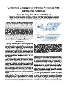
Wireless directional communications methods such as directional antennas and free-space-optical transceivers have become increasingly available.
2
3.1
Classification of research issues in position based routing schemes . . . . 19
3.2
ORRP Basic Example: Source sends packets to Rendezvous node which in turn forwards to Destination . . . . . . . . . . . . . . . . . . . . . . . 20
3.3
1: ORRP Announcements used to generate rendezvous node-to-destination paths 2-3: ORRP RREQ and RREP Packets to generate source-torendezvous node paths 4: Data path after route generation . . . . . . . 25
3.4
ORRP Multiplier Angle Method Parameter Illustration . . . . . . . . . 28
3.5
Basic deviation correction example with Multiplier Angle Method . . . 30
3.6
Multiplier angle method to traverse voids in sparse networks while maintaining direction . . . . . . . . . . . . . . . . . . . . . . . . . . . . . . . 31
3.7
Traversing voids in sparse networks with differing intersection points . . 31
3.8
Forwarding along perimeter is using MAM deals with corner cases where node intersections are outside of topology boundary. Appropriate TTL for ORRP announcement and RREQ packets must be set to minimize excessive state . . . . . . . . . . . . . . . . . . . . . . . . . . . . . . . . 32
3.9
ORRP Reachability for Various Topology Areas: Nodes in darker regions are less reachable. The strength of the darkness of a point shows the probability that a node located on that point will be unreachable by any other node on the area. It can be seen that topology corners and edges suffer from the highest probability of unreach. . . . . . . . . . 36
3.10
Average stretch (ORRP Path/Shortest Path) between two nodes . . . . 38
3.11
ORRP Path vs. Shortest Path Ratio: A node in darker regions have higher likelihood of having longer paths to a destination on the area. Topology corners and edges suffer from the higher stretch in symmetric topologies. . . . . . . . . . . . . . . . . . . . . . . . . . . . . . . . . . . 39
3.12
Average stretch (Frequency distribution of ORRP path stretch in square topology network. Stretch is skewed toward shortest path. . . . . . . . . 40
vii
3.13
Total states maintained in network with respect to the number of transmission lines used. As number of lines increase, the number of states maintained throughout network increases. . . . . . . . . . . . . . . . . . 43
3.14
ORRP reachability, total states maintained, and average path length vs. number of interfaces for dense, average, and sparse networks. In sparse networks, increasing number of interfaces provides significant benefits at first but diminishing returns after 8 interfaces. . . . . . . . . . . . . . 45
3.15
ORRP reachability, total states maintained, and average path length vs. number of interfaces for dense and sparse with large voids present. Small gains can be seen by adding more than 8 interfaces in all cases. . 48
3.16
ORRP reachability, total states maintained, and average path length vs. control packet TTL for various number of interfaces. Increasing TTL up to a certain point does not effect reach probability, states maintained, and average path length. . . . . . . . . . . . . . . . . . . . . . . . . . . 49
3.17
NS2: ORRP Total State Maintained vs. Total Nodes in Network . . . . 50
3.18
NS2: State Maintained in Network Topology. ORRP state is evenly distributed throughout the network. . . . . . . . . . . . . . . . . . . . . 50
3.19
Reach probability, total states maintained, and average path length vs. number of lines used for transmissions for dense and sparse with no voids present. As expected, as number of lines increased, the reach probability and total states maintained increased while average path length decreased. . . . . . . . . . . . . . . . . . . . . . . . . . . . . . . 52
3.20
Reach probability, total states maintained, and average path length vs. number of lines used for a rectangular topology. Reach is drastically affected by additional lines due to better paths in a slim topology. . . . 53
3.21
Reach probability, total states maintained, and average path length vs. number of lines used for transmission for dense and sparse topologies with large voids present. As expected, with voids present, paths taken should be relatively equal due to less choices. At the same time, as more lines are used, the reach probability and total states maintained increased. . . . . . . . . . . . . . . . . . . . . . . . . . . . . . . . . . . . 54
3.22
Average throughput increases as number of lines increase. It can be seen that throughput is largely dependent on average hop count: as average hops increase, the throughput drops. . . . . . . . . . . . . . . . 56
viii
3.23
Packet delivery success and average path length vs. number of nodes in the network for various routing protocols. It can be seen that with more lines, ORRP delivers more packets with shorter average path length. Because AODV and DSR utilize shortest path algorithms, it is expected that average path length is smaller compared to ORRP. . . . . . . . . . 59
3.24
Control packets received and average throughput vs. number of nodes in the network for various routing protocols. ORRP with more lines sends out more control packets as expected. Because ORRP is a hybrid proactive/reactive protocol, it is expected to disseminate more packets than DSR and AODV. Throughput is very much dependent on average path length. . . . . . . . . . . . . . . . . . . . . . . . . . . . . . . . . . 60
3.25
Data delivery success and average path length vs. number of connections. As connections increase, it can be seen that the network becomes saturated faster with AODV and DSR. Average path length is fairly constant throughout. . . . . . . . . . . . . . . . . . . . . . . . . . . . . 61
3.26
Total control packets received and average throughput vs. number of connections. With more connections, more control packets and congestion result in throughput drops. . . . . . . . . . . . . . . . . . . . . . . 62
3.27
Delivery success ratio, aggregate network goodput, and average packet latency measurements for ORRP as compared to DSR and AODV . . . 62
3.28
Reach probability and average path length vs. number of lines used for transmission for mobile networks. ORRP was never designed for mobility but as it can be expected, addition of lines increases reach probability. This is most likely due to shorter paths chosen. . . . . . . . 65
4.1
Basic MORRP Example: Source sends to rendezvous node R found in region illustrated which in turn sends to destination D found in the DRT region given. . . . . . . . . . . . . . . . . . . . . . . . . . . . . . . 67
4.2
Directional Routing Tables (DRTs) map a direction to a set-of-IDs stored in bloom filters . . . . . . . . . . . . . . . . . . . . . . . . . . . . 69
4.3
Each interface has a different relative notion of how fast a specific node is traveling. . . . . . . . . . . . . . . . . . . . . . . . . . . . . . . . . . 72
4.4
Each interface/transceiver has a specific coverage region. As a node moves in one direction, the spread overflows to regions covered by neighboring interfaces. . . . . . . . . . . . . . . . . . . . . . . . . . . . . . . 74
4.5
MORRP neighbor information is decayed going farther and farther from the source. . . . . . . . . . . . . . . . . . . . . . . . . . . . . . . . . . . 75
ix
4.6
1: MORRP Announcements used to generate rendezvous node-to-destination paths 2-3: MORRP RREQ and RREP Packets to generate source-torendezvous node paths 4: Data path after route generation . . . . . . . 80
4.7
MORRP reachability numerical analysis calculation . . . . . . . . . . . 87
4.8
MORRP reachability vs. max mobility speed for various decay factors. As time decay factor increases, reach probability drops due to confusing paths as old information is not decayed adequately. As distance decay factor increases (more bits dropped per hop), a plateau in reach occurs. Reach probability peaks at roughly 6 bits (20% of hash functions) as near and far-field threshold is increased. . . . . . . . . . . . . . . . . . . 91
4.9
Far-field DRT dependence vs. various decay factors. It can be seen that as more bits are dropped, more dependence on the far field occurs. . . . 92
4.10
MORRP reachability, average path length, and far-field DRT dependence vs. spread decay ratio for various mobilities. As spread decay is increased, less bits are dropped but rather “spread” to surrounding interfaces. The lack of bits being dropped leads to confusing path selection yielding in less reach. In this example, both near-field and far-field DRTs used spread decay . . . . . . . . . . . . . . . . . . . . . . . . . . 94
4.11
MORRP reachability, average path length, and far-field DRT dependence vs. spread decay ratio for various mobilities where spread decay is used for only the far-field DRT. Under average network density, spread decay helps reach probability by roughly 1-2% when applied at a ratio of 0.6. Path length, however, is increased. . . . . . . . . . . . . . . . . . 95
4.12
MORRP yields above 90% reachability (data delivery success) even in highly mobile environments. Average path length is fairly equal compared to the other protocols and latency is low because of the more efficient use of the medium in finding a path. . . . . . . . . . . . . . . . 96
4.13
MORRP fairs poorly under low network density but as network density increases, MORRP scales much better . . . . . . . . . . . . . . . . . . . 97
4.14
MORRP maintains fairly low packet overhead even in highly mobile environments. . . . . . . . . . . . . . . . . . . . . . . . . . . . . . . . . 98
4.15
MORRP achieves high aggregate throughput because of high reachability. 99
A.1
ORRP unreachability probability calculation . . . . . . . . . . . . . . . 114
x
ACKNOWLEDGMENT This material is based upon work supported by the National Science Foundation under Grant Nos. IGERT 0333314, ITR 0313095, and STI 0230787. Any opinions, findings, and conclusions or recommendations expressed in this material are those of the author(s) and do not necessarily reflect the views of the National Science Foundation.
xi
ABSTRACT The increased usage of directional methods of communications (e.g. directional smart antennas [15], Free-Space-Optical transceivers [22], and sector antennas) has prompted research into leveraging directionality in every layer of the network stack. In this thesis, we seek to investigate how the concept of directionality can be used in layer 3 to facilitate routing under contexts of 1) wireless mesh networks, 2) highly mobile environments, and 3) overlay networks through virtual directions. In the context of wireless mesh networks, we introduce Orthogonal Rendezvous Routing Protocol (ORRP), a lightweight-but-scalable routing protocol utilizing the inherent nature of directional communications to relax information requirements such as coordinate space embedding and node localization. The ORRP source and ORRP destination send route discovery and route dissemination packets respectively in locally-chosen orthogonal directions. Connectivity happens when these paths intersect (i.e. rendezvous). We show that ORRP achieves connectivity with high probability even in sparse networks with voids. ORRP scales well without imposing DHT-like graph structures (eg: trees, rings, torus etc). The total state information required is O(N 3/2 ) for N-node networks, and the state is uniformly distributed. ORRP does not resort to flooding either in route discovery or dissemination. The price paid by ORRP is suboptimality in terms of path stretch compared to the shortest path; however we characterize the average penalty and find that it is not severe. In the context of mobile adhoc networks, we introduce Mobile Orthogonal Rendezvous Routing Protocol (MORRP) for mobile ad-hoc networks (MANETs) which tracks node movements based on local information through a novel concept called the directional routing table (DRT) which maps interface directions to a setof-IDs to provide probabilistic routing information based on interface direction. We show that MORRP achieves connectivity with high probability even in highly mobile environments while maintaining only probabilistic information about destinations. MORRP scales well without imposing DHT-like graph structures (eg: trees, rings,
xii
torus etc). We will also show that high connectivity can be achieved without the need to frequently disseminate node position resulting increased scalability even in highly mobile environments. In summary, we provide a framework for utilizing directionality, to solve issues resulting from scalability and high mobility. We show that directional can not only be leveraged to provide adequate routing, but can provide dramatic gains in goodput, end-to-end delay, and network reach.
xiii
CHAPTER 1 Introduction The proliferation of wireless technology in recent years has lead to an explosion of research in cost-effective, self-organizing, and efficient wireless technologies for use by young and old, rich and poor alike. Wireless networks allow for high flexibility in setup and relocation, ubiquitous access, and ease of use at the cost of lower throughput (due to interference, a high-loss medium, and limited available spectrum) and weakened security (anyone within range can intercept the signal). The rapid deployment of broadband wireless systems such as 802.11 wireless local area networks (WLANs), 802.16 wireless broadband and neighborhood area wireless networks, however, raises concerns in scalability. In short, as networks become larger and denser, capacity issues arise from the inherent broadcast nature of the wireless medium and limited unlicensed spectrum available to use at any given time.
Figure 1.1: Directional antennas utilize the medium much more efficiently
Researchers have tackled the issue of scalability at all levels of the network stack through novel methods such as adjusting transmit power (to minimize interference with neighboring nodes), scheduling coordination (to assure fair use of the medium), increasing diversity through different modulation, coding, and antenna 1
2 alignment techniques, among others. More recently, there has been a lot of work on utilizing directional antennas to increase network capacity and efficient medium usage. Figure 1.1 shows the obvious motivation: using traditional omnidirectional antennas, as the network becomes denser, simultaneous transmissions quickly saturate the network. With directional antennas, however, the limited scope of the transmission allows the medium to be shared more efficiently. In addition, directional antennas have been shown to provide more reliable transmission across the board. Previous work in directional antennas focused heavily on measuring network capacity and medium reuse [15] [16]. In these works, it was shown that with proper tuning, capacity improvements using directional over omnidirectional antennas are 4π dramatic - ranging from a factor of √2π for planned networks to a factor of √ αβ
2
αβ
for random networks where α and β are the beamwidths of the transmitting and receiving antennas.
Figure 1.2: Wireless directional communications methods such as directional antennas and free-space-optical transceivers have become increasingly available.
Another way to scale networks is to increase network capacity. If the pipe is larger, it becomes easier to push more information through. In effort to increase bandwidth on wireless transmissions, researchers in recent years have been inves-
3 tigating free space optical (FSO) communications technologies as a compliment to traditional RF methods. Currently available in point-to-point links in terrestrial last mile applications and in infrared indoor LANs [45] [44], FSO has several attractive characteristics like (i) dense spatial reuse, (ii) low power usage per transmitted bit, (iii) license-free band of operation, and (iv) relatively high bandwidth compared to RF. Conversely, FSO suffers from (i) the need for line of sight (LOS) alignment between nodes and (ii) reduced transmission quality in adverse weather conditions. [?] proposed several ways to mitigate these issues by tessellating low cost FSO transceivers in a spherical fashion (see Figure 1.2) and replacing long-haul point-topoint links with short, multi-hop transmissions. Given the seemingly large increases in medium reuse and potential for higher bandwidth in directional forms of communications, it becomes interesting to investigate how directionality can be used to facilitate and even improve wireless networks in all layers of the stack. There are several challenges associated with using directionality in mobile networks. Unlike omnidirectional antennas where neighbor reach depends almost exclusively on range, nodes using directional antennas need also take into account the neighbor’s direction and map it to a specific interface in that direction. The problem is complicated even further as nodes closer to a source seemingly incur more dynamism (even small movements can affect perceived direction dramatically) while nodes farther away incur less change. Prior work in directional antennas and FSO technologies have focused on issues with the physical and MAC layer (Layer 1 and 2). Our intent is to explore how directionality can be used in the network layer (Layer 3) to route packets scalably even in highly mobile environments. Routing in multi-hop wireless networks involves the indirection from a persistent name (or ID) to a locator and has grappled with the twin requirements of connectivity and scalability. Early MANET protocols such as DSR [10], DSDV [8], AODV [9], among others, explored proactive and reactive routing methods which either flood information during route dissemination or route discovery, respectively. Many improvements to existing protocols call for either limited link state dissemination [12, 31], limited route maintenance [108, 109], or complex hierarchical struc-
4 tures [11] which all continue to rely on flooding to a certain degree. Even in mesh networks which are not mobile, link-states need to be flooded more often than in wired networks. Flooding poses an obvious scalability problem. In response, position-based routing paradigms such as GPSR [3] were proposed to reduce the state complexity and control-traffic overhead by leveraging the Euclidean properties of a coordinate space embedding. These schemes require nodes to be assigned a coordinate in the system, and still require a mapping from nodeID to coordinate location. In this thesis, we will show that directionality can be used in the network layer (Layer 3) to provide efficient, unstructured, and scalable routing possibilities without flooding (as many topology-based routing protocols do) and without the need for explicit positioning (as with all position-based routing protocols). We will show that our work not only applies to wireless mesh and mobile adhoc networks, but can also be abstracted to virtual overlay networks and even wired ethernet through novel concepts such as virtual directions to limit the scope of flooding.
1.1
Research Objectives In this work, we propose and study mechanisms at the network layer that
use the concept of directionality to route information in a scalable, unstructured manner. Beginning with a basic idea in a fixed wireless mesh scenario, we extend our work to mobile ad-hoc networks, and finally abstract it even further to overlay networks through the concept of virtual directions. This subsection identifies and illustrates the goals and current contributions in each of these cases. 1.1.1
Fixed Wireless Mesh Context Objectives Wireless mesh networks have attracted interest in the research community be-
cause they can complement the cellular model and expand wireless reach in metrobroadband deployment [28]. Their fixed nature, ability to self organize and coordinate, lack of power and processor constraints, and potential to provide ubiquitous wireless access make wireless mesh networks a highly attractive option in providing last mile wireless access. In recent years, several individual communities have setup
5 easy-to-use community wireless mesh networks as an alternative to wired setups and infrastructure base stations. While there has been quite a bit of excitement for the wireless mesh paradigm, only recently has large scale deployment been considered. Because of their fixed nature and highly available processing and power resources, research in wireless mesh networks in the network layer has focused heavily on providing high throughput, low latency, and low load end-to-end paths while keeping control overhead to a minimum. Routing metrics such as expected hop count (ETX) have replaced traditional the “next hop” concept in wireless networks as the defacto standard for evaluating the quality of a wireless link and has led to many routing paradigms built to maximize these routing metrics. As wireless mesh networks grow in size and density, however, scalability becomes a more pressing problem. Even maintaining paths from every source to every destination incurs significant overhead because traditional routing protocols flood the network either in route discovery or dissemination phases. Researchers have addressed the issue of scalability in wireless mesh networks through novel methods that limit flooding network-wide by adjusting dissemination TTL [31, 12], building hierarchical structures [11], employing hybrid proactivereactive approaches [34], and using MAC backoff timers to perform routing without routes [108, 109, 110]. Even then, however, the broadcast nature of the wireless medium necessitates flooding more often than in wired networks. Flooding, even on a limited scale, poses an obvious scalability problem. In response, position-based routing paradigms such as GPSR [3] were proposed to reduce the state complexity and control-traffic overhead by leveraging the Euclidean properties of a coordinate space embedding. These schemes require nodes to be assigned a coordinate in the system, and still require a mapping from nodeID to coordinate location incurring additional overhead. Given the promising future of directional communications as a compliment to traditional RF omnidirectional methods, we propose to investigate how directionality can be used in layer 3 routing without the need for flooding either in the route dissemination or discovery phase. Specific objectives include: • Protocol Development - We intend to develop a routing protocol that uti-
6 lizes the inherent nature of directionality to relax assumptions in positionbased schemes such as the need for coordinate space embedding and locationto-ID mapping. • Protocol Analysis - We intend to show that a) even with directional forms of communications which inherently limit reach, high reachability can be acheived without flooding, b) Average states maintained network-wide scales reasonably well, c) path stretch vs. shortest path is not bad. • Protocol Evaluation - We intend to evaluate our protocol against current routing protocols using the metrics of data delivery success, total state maintenance, average path length, end-to-end latency, aggregate network goodput, and control packet overhead under conditions of varying node density, number of interfaces, control packet TTL, and network topologies. 1.1.2
Mobile Adhoc Network Context Objectives There are several challenges associated with using directionality in mobile
networks. Unlike omnidirectional antennas where neighbor reach depends almost exclusively on range, nodes using directional antennas need also take into account the neighbor’s direction and map it to a specific interface in that direction. The problem is complicated even further as nodes closer to a source seemingly incur more dynamism (even small movements can affect perceived direction dramatically) while nodes farther away incur less change. With protocols reliant on directionality, it is easy to see how mobility can easily disrupt routes because node movement affects routing state much more frequently. It is therefore interesting to investigate how directionality can be applied in layer 3 routing in highly mobile environments. To that end, we propose the following objectives: • Protocol Development - We intend to develop a protocol that uses directionality to solve issues caused by high mobility in mobile adhoc networks (MANETs). • Protocol Analysis - We intend to analyze our protocol to understand the limitations of the scheme including reach probability in high mobility and total
7 control overhead. • Protocol Evaluation - We intend to compare our protocol with existing MANET protocols under highly mobile environments to understand the tradeoff in reachability, total states maintained, control packet overhead, end-to-end latency and aggregate network throughput. 1.1.3
Overlay Network Context Objectives Overlay networks such as peer-to-peer systems have blossomed in recent years
for their ability to link and share media files across the internet ubiquitously. Overlay networks are computer networks built on top of other network. Nodes in an overlay network can be thought of as being connected by virtual or logical links irrespective of the underlying network. One of the biggest challenges of virtual networks like peer-to-peer systems is scalability. Efforts to mitigate flooding for content search all including building set structures to hash content to and performing a search based on a hashing structure. In this work, we seek to investigate whether the concept of directionality can be applied to overlay networks and abstracted to virtual directions. Mapping content and nodes to virtual directions allows us to be able to employ techniques from the previous sections to perform searches in a scalable, non-flooding manner. We propose the following objectives: • Concept Development - We intend to explore how nodes in an overlay network such as peer-to-peer or ethernet can be abstracted to the concept of virtual directions that are globally consistent without the need for flooding. • Employ Prior Techniques to Limit Flooding - We intend to apply previous techniques developed in using directionality for wireless networks to evaluate the viability of using virtual directions in overlay networks.
1.2
Research Contributions In this section, we present our contributions thus far in each of the contexts
listed above.
8 1.2.1
Fixed Wireless Mesh Context Contributions In our work, we present Orthogonal Rendezvous Routing Protocol (ORRP), a
layer 3 routing protocol using characteristics inherent to directional communications, to forward packets. ORRP is based upon two simple ideas: a) local directionality is sufficient to maintain forwarding of a packet on a straight line, and b) two sets of orthogonal lines in a plane intersect with high probability even in sparse, bounded networks. ORRP assumes that each node has directional communication capability and can therefore have a local sense of direction (i.e. orientation of neighbors is known based on a local North). Notice that this is an even weaker form of information than a global sense of direction (i.e. orientation of neighbors is known based on a global North) which necessitates additional hardware such as a compass. We show through analysis and performance evaluations that: • ORRP achieves high connectivity ( 98%) even in sparse networks with voids. • ORRP state scales on the order of O(N 3/2 ) and the state is distributed fairly evenly network-wide providing no single point of failure • ORRP does not flood during route discovery or dissemination and coupled with the inherent nature of directional communications, yields over 20x the aggregate network goodput compared to DSR and AODV. • Although ORRP paths are suboptimal compared to shortest path, our analysis shows that the path stretch is not bad ( 1.2) and that the end-to-end latency generated by these paths coupled with more efficient medium reuse lends itself to much lower end-to-end delays than in DSR and AODV. 1.2.2
Mobile Adhoc Network Context Contributions Heavily extending our previous work, we present Mobile Orthogonal Ren-
dezvous Routing Protocol (MORRP) which leverages directionality and probabilistic routing to route packets in highly mobile environments without the need to frequently disseminate information. MORRP facilitates high mobility by abstracting the concept of rendezvous points to rendezvous regions and forwards packets probabilistically based on which direction a destination or rendezvous node is most likely
9 found. These directions shift accordingly to a node’s local velocity. For example, if a source node is moving north, a node originally east of the source will seem to be moving south. We introduce a novel concept called the directional routing table (DRT) which replaces traditional routing tables. The key contributions of MORRP include: • Using directionality to solve the issues caused by high mobility in MANETs - Using only local information, any node is able to more efficiently “guess” the direction of a destination and forward probabilistically. • The Directional Routing Table - A replacement for traditional routing tables based on purely probabilistic routing. DRTs map a specific direction to a set-of-IDs which eliminates the need to maintain exact routing information about nodes in a network while lessening the frequency of route dissemination. • Routing Based on Probabilistic Hints - Traditional routing protocols have a hard limit on route expiration. With probabilistic routing, routing information is decayed with time and becomes less and less accurate. Below a certain threshold, the information becomes insignificant. In our performance evaluations, we show that: • MORRP yields above 90% reachability even in highly mobile environments accounting for an almost 50x higher aggregate goodput compared to DSR and AODV. These gains come by using directionality constructively and scalably to overcome problems inherent with directionality. • End to end packet latency is very low under MORRP compared to DSR and AODV because of more efficient medium reuse. • As node density increases, DSR and AODV data delivery success drops significantly due to network saturation but does not affect MORRP much. • MORRP sends slightly more control packets than ORRP but significantly less than DSR and AODV in highly mobile situations.
CHAPTER 2 Literature Survey The growth of the internet has raised important questions regarding the scalability of computer networks. At first, flooding-based approaches were the norm. As networks began to grow in size and complexity, however, new approaches to limit flooding were necessary. Hierarchical-based approaches to address scalability were heavily examined as a result. More recently, there has been a push to use primitives such as local information and random walks to scale flat networks in an unstructured way. Given the trends in utilizing directional communications, we believe that an important way to scale large flat networks is through using directionality. In this chapter, we will examine related work on how routing protocols have scaled in the past and how directionality has changed the game.
2.1
Scaling Wireless Routing Protocols There has been a considerable amount of work on wireless routing protocols
in recent years. Classified into five major types (reactive, proactive, hierarchical, position-based, and hybrid of the approaches), these protocols rely on different assumptions and tradeoff different metrics like connectivity, path selection, state maintenance, etc. to route packets through a network. Reactive protocols like AODV [9] and DSR [10] perform route discovery by flooding the network and delay data from being sent until a route is found. While considerably less state needs to be maintained at each node, route-discovery flooding of the entire network can be costly and inefficient. By contrast proactive protocols like DSDV [8] and OLSR [31] periodically broadcast routing information across the network (or in certain areas of the network), and maintain extensive routing tables at each node. Each data packet references the routing table of every hop in the packet and forwards accordingly. In much the same way as reactive protocols, heavy network floods of control packets incur high overhead and can be inefficient. As a response to to apparent issues with scalability of traditional reactive and 10
11 proactive protocols, hierarchical and position-based approaches were examined heavily. Hierarchical routing protocols such as HRP [11], LANDMAR [26], and L+ [32] splice the network into regions that maintain routing information within the area. Certain nodes within each region are selected to be gateway nodes which maintain overlay routing tables with gateway nodes from other regions. Thus, routing within each region happens normally while routing inter-region is handled by the gateway node. While an important step in achieving greater scalability, hierarchical routing techniques rely too heavily on the special nodes that maintain routing between regions, and increased complexity of reorganization make it harder to implement. Recently, there has been a new push toward a new type of routing paradigm for wireless sensor networks that utilizes MAC backoff timers and the broadcast medium of wireless to self-route packets without maintaining routing tables. Self-Selective Routing (SSR) [110, 109, 111] and Self-Healing Routing (SHR) [108, 107] are examples of this class of routing protocols. After an initial flood-based ”number of hops to destination” request is performed, subsequent packets are forwarded with next hops determined after the packet has been sent. Local leader selection techniques for MAC backoff timers based on the distance in hop count from the destination are implemented to choose a next hop to take the packet forward. While effective in situations where node failures are high such as in sensor networks because routes do not need to be maintained, SSR and SHR still uses flooding to find initial paths and rely on hop count to determine a “gradient” direction to forward in. As a result, SSR and SHR are not suitable for mobile environments where hop count (and not merely node failure rate) changes dramatically. Position-based protocols like GPSR [3] and TBF [5] tackle the issue of scalability by leveraging geographic position to route packets maintaining little to no state. A packet is forwarded in the “general direction” of the destination until it is reached. While highly scalable in a pure routing-only framework, position-based protocols assume location-to-address mapping techniques such as GLS [4], and node-localization equipment, such as GPS receivers, which incur additional overhead. Hybrid protocols like ZRP [34] and LGF [33] that combine the various strategies add benefits but still suffer from some form of flooding and capacity constraints.
12 In recent years, there has been a big shift from using hierarchical structured schemes, such as GLS [4], which partitions networks into grids that trade location information on a limited basis, to non-hierarchical structured schemes, such as DHT and virtual coordinate-based approaches [37] [36] [35]. DHT/virtual coordinate based approaches such as DPSR [36], VRR [35], among others, build hashes between node IDs and a set structural representation of the nodes. For example, DPSR [36] utilizes fingers that extend from a node while VRR [35] stores hashes in a circular ring format. These unstructured approaches not only effectively remove the need for a positioning system and network flooding, but also makes routing more scalable. The drawback, however, is that paths are suboptimal. D. Braginsky et al. [23] proposed an unstructured rendezvous-abstraction routing technique based on drawing single lines. Events are broadcasted by nodes through random walks and event request packets are sent in a similar way until it intercepts event regions. It was shown that two lines bounded in a rectangle had a 69% chance of intersecting within the rectangle. We see the trend again in routing: moving from flooding, to structured hierarchies, to unstructured techniques to forward packets.
2.2
Scaling using Directional/Sector Antennas Directional and sector antennas have been the object of numerous studies in
the past for their potential in decreasing interference and improving network capacity. Rappaport [102] describes the use of sector antennas on modern cellular base-stations which allows decreasing of the cluster size in order to improve frequency reuse without being afraid of interference. Sectoring even only 120◦ reduces interference significantly and increases capacity by a factor of 1.714. The focus of much of the previous work in directional antennas has been understanding and evaluating its spatial reuse property. Nasipuri et al. [18] modified the RTS and CTS exchange in 802.11 to support directionality and showed through simulations that as a result, a throughput improvement of 2-3 times over omnidirectional antennas. The primary aim of the work was to minimize routing overhead by using directional antenna elements for propagating routing information as routing
13 overheads from omnidirectional transmissions can be costly. Ko et a. [19] proposed directional MAC (D-MAC), a revamp of the current 802.11 MAC scheme to support both directional and omnidirectional operation. The D-MAC scheme showed a throughput boost of about 2 times normal 802.11 operation. Building on top of previous work, Choudhury et. al. [14] designed the MultiHop RTS MAC (MMAC) protocol which uses multi-hop RTS’s to establish links between distant nodes, and then transmits CTS, DATA, and ACK packets over a single hop. Their results show that MMAC outperforms 802.11 but the performance is depending on the topology and flow patterns. Ramanathan [15] evaluates the performance of ad hoc networks with beamforming antennas arriving at several important conclusions: • beamforming antennas yield up to a 118% improvement in throughput and up to a factor of 28 reduction in end-to-end delay in static networks. • Even simple channel access techniques which allow parallel transmissions yield dramatic results. • Link power control is essential in exploiting beamforming antennas • With respect to spatial reuse, switched beams are nearly as good as steered beam antennas. • Directional neighbor discovery is very effective in low densities. Work in measuring capacity gains using directional antennas is not limited to simulation evaluations. Building on network capacity bounds formulated by [?], Yi et al. [16] presents an analytical model for evaluating network capacity using directional antennas. Their work showed that with proper tuning, capacity improvements using directional over omnidirectional antennas are dramatic - ranging from a factor 4π of √2π for planned networks to a factor of √ αβ
2
αβ
for random networks where α and
β are the beamwidths of the transmitting and receiving antennas. Directional antennas not only improve network capacity, but have been shown to be more stable in terms of link quality and not as affected by routing metrics.
14 Chebrolu et al. [21] showed that 802.11 long distance links using directional antennas result in almost “wire-like” characteristics with error rates as a function of the received signal strength behaving close to theory, time correlation of any packet errors being negligible across the range of time-scales, and links being robust to rain and fog. Under such conditions, routing metrics for wireless links become less and less important. More recently, there has been a lot of work showing how current ad hoc routing protocols fail when using directional antennas and how they can be adapted to work using directional antennas. Choudhury et. al. [13] proposes Directional DSR (DDSR), a modification to DSR [10] to address issues with interface handoff, backoff, and neighbor discovery. Gossain et al. [6] presents Directional Routing Protocol (DRP), a cross layer protocol inspired by DSR which handles route discovery, establishment, maintenance, and route recovery mechanisms all using directional antennas. While much of these efforts in using directionality in the routing layer are important, they come more as a response to having directional communications rather than leveraging directionality as a benefit in routing.
2.3
Free Space Optical Communications In recent years, researchers have looked into using free-space-optics (FSO) to
compliment traditional RF networks [50, 22]. Legacy optical wireless, also known as free space optics (FSO), communication technologies use high-powered lasers and expensive components to reach long distances. Thus, the main focus of the research has been on offering only a single primary beam (and some backup beams); or use expensive multi-laser systems to offer redundancy and some limited spatial reuse of the optical spectrum [85, 99]. The main target application of these FSO technologies has been to serve commercial point-to-point links (e.g. [98, 97]) in terrestrial last mile applications and in infrared indoor LANs [93, 99, 92, 91, 90, 94]. Though cheaper devices (e.g. LEDs and VCSELs) have not been considered seriously for outdoor FSO in the past, recent work shows promising success in reaching longer distances by aggregation of multiple LEDs or VCSELs [95, 96]. Another line of work on FSO communications has been on achieving reliable
15 high-speed links for optical interconnects, where auto-alignment or wavelength diversity techniques are reported to improve the misalignment tolerances in 2-dimensional arrays [74, 73, 72, 71, 75, 76]. These techniques work only over small ranges (e.g. 1µm - 1 cm) and some of these are cumbersome involving highly sensitive mechanical tracking instruments. Moreover, they are designed to improve the tolerance to movement and vibration but not to handle mobility. While phased array structures are well known in the RF world, and work in the last decade has made multiple spatial channels possible using smart antenna techniques [69, 70], RF cannot match the high degree of integration and number of spatial channels possible using FSO. For example, a small 1sqft array (smaller than a laptop screen) can allow the integration of around 1000 pairs of transceivers. With each pair operating at 100 Mbps, this can lead to an aggregate backhaul capacity of 100 Gbps! No RF technology can match this performance; expectations of RF techniques with smart antenna techniques in the 5 GHz unlicensed spectrum top off at about 1-5 Gbps. Moreover, RF with spatial arrays (especially in unlicensed bands like 5 Ghz) requires placement of complex, high-speed, mixed signal electronics that would make the unit operate at higher power levels and would be far more expensive. It is interesting to note that today’s laser-based FSO techniques could be extended to form spatial arrays, but such equipment would be very costly and high-power. Moreover, such laser-based equipment would not have the form factor, weight and power characteristics to be mounted on ad-hoc infrastructures like balloons, treetops etc. In addition to the above benefits and potential for spatial integration/spectral reuse, FSO also has critical limits relevant to achieving high-speed communication links. First, FSO requires a clear line-of-sight (LOS) between the transmitter and receiver of a link because these frequencies are absorbed by almost any obstruction (eg: walls, trees, automobiles etc). Though non-LOS optical operation is possible under certain conditions (e.g. indoor infrared [91]), such operation is primarily for short-range, half-duplex LOS (a.k.a Point-and-Shoot (P&S)) links only within a single room (very short distance of 1-10m), expecting the availability of multiple reflected LOS paths. Indoor infrared also requires stringent eye-safety requirements:
16 IEC Class 1 allowable exposure limit (AEL) [66, 67]. The LOS issue has been tackled recently through the use of very low cost components organized in a multi-hop network to get around LOS issues. Akella et al. [103] showed that error characteristics of FSO over multiple hops are very promising. Further, a promising recent trend is the usage of optoelectronic solid-state devices like LEDs for lighting. Packaging of multiple LEDs is shown to be very promising for durable lighting devices and commercializations are taking place for various daily life usage of such solid-state lighting devices [65, 64, 87]. Similar to IrDA deployment in hundreds of millions of devices today, we believe that massive deployment of integrated optoelectronic devices which can illuminate and communicate will provide sufficient FSO-MANET nodes to overcome the LOS problems. In addition, as FSOMANET will be complementary to the traditional RF MANETs, LOS problem will be a secondary problem. The second FSO limitation in regards to high-speed communications is various forms of attenuation. Recall that current FSO links in the field using lasers are limited to a few kilometers [104], though satellite communications has routinely used FSO links ranging several thousands of kilometers. The terrestrial limitations occur primarily due to atmospheric attenuation (e.g., fog, rain, snow) and geometric attenuation (due to beam divergence). Considerable FSO work especially in industry has been on characterizing link availability under various conditions [68, 98, 97], with higher availability in clear-conditions. These studies showed that dense fog affects FSO transmission far more than other conditions, and that an average of 99.98% in all conditions is considered very good availability for FSO. Also, addition of microwave RF backup provides even higher (carrier-class) availability percentages (e.g. 99.999%). The key limitation of FSO regarding mobile communications is the fact that LOS alignment must be maintained for communication to take place successfully. Since the optical beam is highly focused, it is not enough if LOS exists: the transmitter and receiver pair should be aligned; and the alignment must be maintained to compensate for any sway or mobility in the mounting structures. Mobile communication using FSO is considered for indoor environments, within a single room,
17 using diffuse optics technology [91, 93, 100, 89, 88, 87, 86, 84]. Due to limited power of a single source that is being diffused to spread in all directions, these techniques are suitable for small distances (typically 10s of meters), but not suitable for longer distances. For outdoors, fixed FSO communication techniques have been studied to remedy small vibrations [82, 83], swaying of the buildings have been implemented using mechanical auto-tracking [85, 81, 80] or beam steering [79], and interference [78] and noise [77]. LOS scanning, tracking and alignment have also been studied for years in satellite FSO communications [63, 62]. Again, these works considered long-range links, which utilize very narrow beamwidths (typically in the microradian range), and which typically use slow, bulky beam-scanning devices, such as gimballed telescopes driven by servo motors. FSO spherical structures were studied and some of its elementary features such as alignment were built and operated at very short distances and very low speeds [22]. These studies showed promising results and we plan to build several fullystructured prototypes of 3-d FSO spheres which will constitute a lab-based prototype of a demonstrable FSO-MANET working at high speeds and longer communication distances. FSO is very attractive for power-scarce MANET applications such as sensor networks [105]. As discussed earlier, in comparison to RF physical communication characteristics, FSO has critical differences in terms of error behavior, power requirements, etc. Implications of these physical FSO characteristics on higher layers of the networking stack has been studied in recent years. Majority of the FSO research in higher layers has been on topology construction and maintenance for optical wireless backbone networks [61, 60, 59]. Some work considered dynamic configuration [58], node discovery [57], and hierarchical secure routing [56, 55] in FSO sensor networks. However, no deep investigation of issues and challenges that will be imposed on MANETs by FSO has been performed. A key FSO characteristic that can be leveraged at higher layers is its directionality in communication. Though the concept is similar to RF directional antennas, FSO can provide much more accurate estimations of transmission angle by means
18 of its directionality. Previous work (including ours) showed that directionality in communication can be effectively used in localization [106, 54], multi-access control [14, 52], and routing [1, 13, 43, 53, 6]. In addition to directionality, our proposed FSO nodes introduce highly-intermittent disconnectivity pattern (i.e. aligned-misaligned pattern) which affects transport performance [22]. Also, establishment of an FSO communication link implies that the space between the communicating nodes is Euclidian, which can be leveraged to better design routing and localization protocols.
CHAPTER 3 Orthogonal Rendezvous Routing Protocol 3.1
Introduction Wireless mesh networks have attracted interest because they can complement
the cellular model and expand wireless reach in metro-broadband deployment [28]. Routing in multi-hop wireless networks has grappled with the twin requirements of connectivity and scalability. Early MANET protocols such as DSR [10], DSDV [8], AODV [9], among others, explored proactive and reactive routing methods which either flood information during route dissemination or route discovery, respectively. Improvements such as SSR [109] and SHR [108] which uses MAC backoff timers to do local leader selection after packets have been sent to limit route maintenance still rely on a flood-based initial route discovery. Even in mesh networks which are not mobile, link-states need to be flooded more often than in wired networks. Flooding poses an obvious scalability problem. In response, position-based routing paradigms such as GPSR [3] were proposed to reduce the state complexity and control-traffic overhead by leveraging the Euclidean properties of a coordinate space embedding. These schemes require nodes to be assigned a coordinate in the system, and still require a mapping from nodeID to coordinate location. In this paper, we focus on routing with even less information, i.e. scalable, efficient routing without explicit positioning.
Figure 3.1: Classification of research issues in position based routing schemes A recent trend in wireless communications has been the desire to leverage directional forms of communications (eg. directional smart antennas [15] [13], FSO 19
20 transceivers [22]) for more efficient medium usage and scalability. Previous work in directional antennas focused heavily on measuring network capacity and medium reuse [13] [15] [16]. It has been shown that directional antennas can be used to provide high quality links which tend to be more wire-like and less sensitive to routing metrics [21]. In this chapter, we utilize directionality for a novel purpose: to facilitate layer 3 routing without the need for flooding either in the route dissemination or discovery phase. Our protocol, called Orthogonal Rendezvous Routing Protocol (ORRP) is based upon two simple ideas: a) local directionality is sufficient to maintain forwarding of a packet on a straight line, and b) two sets of orthogonal lines in a plane intersect with high probability even in sparse, bounded networks. ORRP assumes that each node has directional communication capability and can therefore have a local sense of direction (i.e. orientation of neighbors is known based on a local North). Notice that this is an even weaker form of information than a global sense of direction (i.e. orientation of neighbors is known based on a global North) which necessitates additional hardware such as a compass. Figure 3.2 illustrates an example operation of ORRP.
Figure 3.2: ORRP Basic Example: Source sends packets to Rendezvous node which in turn forwards to Destination
Consider a source node S that wishes to send packets to a destination node D. Both nodes S and D have their own local notions of orientation. Source S sends
21 route discovery packets in four orthogonal directions and the destination D does likewise for route dissemination packets. The route discovery packets will rendevous at a node touched by a route dissemination packet at up to two rendezvous points on the plane. We refer to the intersection that facilites a shorter path as the rendezvous node R. Node R directs packets from source S to the destination D. Node D’s state is only maintained on the two orthogonal lines, which implies that the total state complexity is O(N 3/2 ) for an network of N nodes. If each node chooses its local orthogonal directions independently, ORRP state information is fairly evenly distributed throughout the topology resulting in no single point of failure. Further, there is no flooding by either source S or destination D. All these factors enable scalability without imposing the requirement of an explicit hierarchical structure [4, 11]. In other words, ORRP offers a scalable, unstructured indirection method for routing in contrast to the hierarchically structured methods suggested in prior work. However, the ORRP paths chosen are suboptimal, i.e. have a stretch factor greater than 1 compared to the corresponding shortest paths. However, we show that this factor is not too large on average. The rest of this chapter is organized as follows: We first outline key design issues of ORRP in the next subsection. Section 3.2 deals with the specifics of ORRP including assumptions, concepts and examples. Section 3.3 provides performance analysis including basic Matlab simulations to formulate upper bounds on reachability and average shortest path while section 3.4 examines these issues in more realistic packetized simulation environments. 3.1.1
Key Design Considerations To fully realize the implications of ORRP, it is important to understand what
issues traditional geographic routing protocols face. The problem of end-to-end wireless geographic routing using network localization can be broadly categorized into three layers as shown in Figure 3.1. The lowest layer L1 is the localization scheme that obtains node coordinates [4] [2] while the second layer L2 maps these coordinates to node “identifiers” like a name or a number. Once these two are established, the third layer L3 uses this information to perform geographic routing.
22 Current research in geographic routing protocols (e.g. GPSR [3], TBF [5], GLS [4], Landmark [26]) often tackle one of the three layers and assume the others to be a given. When taken separately, schemes in each layer can be shown to be extremely scalable. However, combining the effects of maintenance of the three layers can be rather costly. ORRP provides a simple, lightweight alternative to tackle layers L2 and L3 while removing the need for layer L1 all-together. Specifically, ORRP focuses on and attempts to optimize based on the following considerations: • Connectivity Under Less/Relaxed Information compared to Position-based Protocols - Position-based protocols such as GPSR [3] or TBF [5] operate under the assumption that each node has a globally consistent view of its own as well as other’s geographic positions. ID-to-location mappings (location discovery problem) are assumed to be a given. While this assumption is appropriate given the lowering cost of GPS receivers and several proposed methods of solving the location discovery issue [24, 25], maintaining global view of the network in this way can be costly, unavailable (e.g. GPS receivers need “sky access” and cannot be used indoors) and might not be scalable in larger or highly dynamic networks. ORRP eliminates the need for location discovery by utilizing the fact that two pairs of orthogonal lines mostly have intersection points. These “rendezvous points” act as forwarders of data increasing scalability. • Efficient Medium Reuse - Topology-based routing protocols often fall into two camps: proactive (e.g. DSDV [8]) and reactive (e.g. DSR [10], AODV [9]). Proactive protocols consistently flood the network with control packets to maintain up-to-date routing tables at each node. While this ensures high packet delivery success even in mobile environments, scalability is limited due to the sheer number of control packets needed to maintain up-to-date routing tables. Reactive protocols attempt to solve this issue by requesting routes “on demand” and then caching those routes. While this works for less mobile environments, similar issues with scalability arise. ORRP mitigates these issues by forwarding control packets proactively only in orthogonal directions thereby
23 freeing the medium for data, and then reactively requesting routes when one is not cached and is needed. These route requests do not flood the network unnecessarily because they are transmitted only in orthogonal directions and once a rendezvous node receives these request packets, it stops the forwarding. • Less State Information Needed to be Maintained - Because ORRP only maintains routing information in orthogonal directions, scalability is increased. In order to optimize and bring out the advantages listed above, there are several tradeoffs associated with ORRP: • Increased Path Stretch - ORRP optimizes connectivity and efficient medium reuse with little agreed-upon information. The cost of less information is that packets often take paths longer than shortest path. We will show that although ORRP paths are suboptimal, under normal circumstances, the average path stretch is close to optimal. • Limited Reachability - Due to possibility of no intersection of orthogonal lines, some source and destination pairs might not have rendezvous points resulting in unavailable paths. While several corrective measures are suggested in ORRP, we will show that under normal operation, the packet delivery success is extremely high.
3.2
ORRP: Basic Scheme and Design Parameters In this section, we will detail the assumptions, specifications, and mathemat-
ical aspects of ORRP. Specifically, we will 1) address assumptions made by ORRP including hardware requirements and other cross-layer abstractions, 2) detail the proactive and reactive elements of ORRP, and 3) explain path deviation correction and void traversal with the Multiplier Angle Method (MAM). 3.2.1
Assumptions ORRP relaxes many of the assumptions made by position-based routing proto-
cols while still providing high connectivity. ORRP makes no assumptions on location
24 discovery and uses packets forwarded in orthogonal directions to find paths to the destination from a given source. To do so, ORRP makes three major assumptions: • Neighbor Discovery - We assume that any given node will know (i) its 1-hop neighbors and (ii) the given direction/interface to send packets to reach this neighbor. • Local Sense of Direction - Each node must have its own local perception of direction (i.e. each antenna/transceiver knows its own orientation with respect to the “local north”). • Ability to Transmit/Receive Directionally - Nodes must be capable of communicating directionally over their transceivers. This can be done by various hardware including directional and smart antennas [13], and FSO transceivers [22]. FSO transceivers are a particular interest due to their fine-grained transmit angle and ability for several dozen to be tesselated together oriented in several directions on a single node [22]. 3.2.2
Theory The basic concept behind ORRP is simple: knowing that in 2-D Euclidian
space, a pair of orthogonal lines centered at different points will intersect at two points at minimum, rendezvous points can be formed to forward packets as shown in Figure 3.2. To achieve this, ORRP relies on both a proactive element which makes up the “rendezvous-to-destination” path and a reactive element which builds a “sourceto-rendezvous” route on demand. Nodes periodically send ORRP announcement packets in orthogonal directions and at each node along the orthogonal route, the node stores the route to the source of the ORRP announcement and the node it received the announcement from (previous hop). When a source node wishes to send to some destination node that it does not know the path for, it sends out a route request packet (RREQ) in its orthogonal directions and each subsequent node forwards in the opposite direction from which it receives the packet. Once a node containing a path toward the destination receives an RREQ, it sends a route reply packet (RREP) in the reverse direction back to the sender and data
25 transmission begins. In the following subsections, we will detail and explain the tradeoffs associated with each element of ORRP. 3.2.2.1
Proactive Element
Figure 3.3: 1: ORRP Announcements used to generate rendezvous nodeto-destination paths 2-3: ORRP RREQ and RREP Packets to generate source-to-rendezvous node paths 4: Data path after route generation In order for a source and destination to agree upon a rendezvous node, preestablished routes from the rendezvous node to the destination must be in place. Because each node has merely a local sense of direction, making no assumption on position and orientation of other nodes in the network, it can only make forwarding decisions based on its own neighbor list. After a set interval, each node sends ORRP announcement packets to its neighbors in orthogonal directions as shown in Figure 3.3. When those neighbors receive these ORRP announcement packets, it includes the source, previous hop, and hop count into its routing table as a “destination-next-hop pair” and forwards it out the interface exactly opposite in direction from the interface it received the packet. Although we currently only consider hop-count to be the metric for path selection, it is easy to adapt ORRP to use other heuristics such as ETX [29] among others. It is important to note that each node does not maintain a complete picture of the network which limits the state information needed to be updated, and
26 thereby increasing scalability. Moreover, only forwarding in orthogonal directions provides enhanced medium reuse. Based on mobility speeds, energy constraints, and other factors, parameters that can be tweaked for higher performance of ORRP announcements include announcement send interval and forwarding entry expiry time. Because the forwarding table only maintains information about destination and next hop, overhead in storage and maintenance is minimized as well. 3.2.2.2
Reactive Element
In order to build the path from source to rendezvous node, an on-demand, reactive element to ORRP is necessary. When a node wishes to send packets to an destination that is not known in its forwarding table, it sends out a route request packet (RREQ) in all four of its orthogonal directions. When neighbor nodes receive this RREQ packet, it adds the reverse route to the source into its routing table and forwards in the opposite direction. In a 2-D Euclidian plane, by sending a RREQ packet in all 4 of its orthogonal directions, it is highly likely to encounter a node that has a path to the destination. When a node with a path to the destination receives the RREQ, it sends a RREP packet back the way the RREQ came. Because each node along the path stored a reverse route to the source, it is able to forward the RREP back efficiently after recording the “next-hop” to send to this particular destination. When the source receives the RREP, it generates a “destination-next-hop” routing entry and forwards packets accordingly. Figure 3.3 illustrates the process of sending RREQ and RREP packets while showing the ORRP path selected. Unlike AODV, DSR or other reactive protocols, RREQ packets are not forwarded until they reach the destination, but only until it intersects a rendezvous node. The proactive element of ORRP takes care of the rendezvous node-to-destination path. It is important to note that ORRP path is not equivalent to the shortest path for most cases. As mentioned earlier, we gained connectivity under relaxed assumptions at the cost of suboptimal path selection (increased path stretch). We will show later, however, that the path selection is close to optimal resulting in a
27 fairly nonexistent cost. 3.2.2.3
Deviation Correction: Multiplier Angle Method
Up until now, we have considered only situations where nodes forward in orthogonal directions assuming that neighbors are all aligned on a straight line. In reality, however, straight line paths in random networks rarely exist. Although ORRP works on path intersections and as a result, does not need to enforce the rule that packets sent in orthogonal directions must remain true to their path, upholding this rule increases the probability of finding intersections. [23] shows that that two straight lines randomly drawn in a euclidian plane have a 69% chance of intersecting within a given area. We will show in later sections that two pairs of orthogonal lines have a 98% chance of intersecting. To address the deviation issue, it is important to clarify a few key concepts and limitations. First, deviation corrections can only be done when the deviation is greater than the conical spread of the directional antenna or transceiver. Interfaces oriented in a circular fashion, so that each of the antennas attached to a particular node operate at a set angle from the local “north”, have a coverage much like a pizza pie. Depending on the beam width and assuming no overlap in spread, a node can be at various degrees of deviation from the actual orientation of each particular antenna even though it is within the beam spread/coverage area. ORRP does not deal with deviations that occur within one antenna coverage area. Next, ORRP assumes that the relative distances from one hop to another are relatively equal. In dense networks, this is a safe assumption due to the sheer volume of nodes. It will be shown that sparse networks do not care about distances either way due to lack of nodes. Finally, all deviation corrections are done at the RREQ and ORRP announcement level so that data transmission does no such calculations per hop. ORRP addresses the issue of deviation correction by a multiplier angle method (MAM). Each RREQ and ORRP announcement packet has an additional field in the packet header: deviation multiplier. For simplicity, we assume that all nodes have equal number of transceivers each separated with equal distances. The deviation
28 multiplier is used to calculate the deviation angle from the desired angle at which a packet was sent. Table 3.1 defines a few key parameters which are illustrated in Figure 3.4.
Figure 3.4: ORRP Multiplier Angle Method Parameter Illustration
Table 3.1: Multiplier Angle Method Definitions Received Angle (γ)
The angle node received packets from. Deviation Angle (θ) The angle to add/subtract in order to correct the deviation. Desired Angle (α) The desired angle to send out. Found Angle (β) The angle of transceiver found cloest to desired angle with neighbor nodes. Separation Angle (τ ) The angle of separation between each transceiver. Multiplier (m) The value to multiply τ by to find new desired angle.
When searching for a next-hop within the corresponding antenna/transceiver beam width, ORRP cycles through all its neighbors and finds one which requires an antenna-deviation angle yet is still confined to less than ±45◦ (if packet is at originator) or ±90◦ (if packet is merely a forwarder) of the original direction. If a packet is at the originator, only ±45◦ needs to be searched because each of the four orthogonal directions is sending. So, giving each direction a 90◦ coverage effectively
29 covers all directions. In the forwarding case, however, because only one direction is considered with potentially “void” spots, a greater angle range is given to traverse “voids” yet ensure packets are not forwarded directly the opposite direction. If no neighbor is found satisfying these conditions, the packet is dropped and an error is flagged. The following equations are used to calculate angle to send and what state to store in each packet (all angle values are between 0◦ and 360◦ ): π Dev Angle θ = min(+ , 2 ∗ (τ ∗ m)), m positive 2
(3.1)
π Dev Angle θ = max(− , 2 ∗ (τ ∗ m)), m negative 2
(3.2)
Desired Angle α = γ + π − θ
(3.3)
M ultiplier m =
(β − α) τ
(3.4)
At each hop, the node unpacks the multiplier from the packet header and calculates a desired angle to send out based on (3.3). It then searches through its neighbors which have corresponding transceiver angles and finds one with the closest angle to the desired angle. When one is found, a new multiplier is calculated based on (3.4) and stored into the forwarding packet header before the packet is sent out. The process is repeated until the packet arrives at the destination. Algorithm 1 breaks down the process step-by-step. Algorithm 1 Multiplier Angle Method 1: Unpack old multiplier m 2: Calculate angle needed to correct deviation θ (From eqs 3.1 and 3.2) 3: Calculate desired angle α (Eq 3.3) 4: Find interface with direction closest to α that has a neighbor (found angle β) 5: Calculate new multiplier m (Eq 3.4) An example of our proposed multiplier angle method for deviation correction is shown in Figure 3.5. Node S is sending packets along the line. Because it has no nodes along the line in range of its transceivers, S opts to send to node A which is at a transceiver angle of τ from the desired angle α and encode multiplier m of one into the packet header. When node A receives S’s packet, it calculates the desired
30
Figure 3.5: Basic deviation correction example with Multiplier Angle Method outgoing interface based on (3.3) and as a result, sends to Node B while encoding a multiplier m of zero because there is no deviation from desired angle and found angle. The rest is self explanatory. Potential problems may arise if the problem is cascading: Suppose node A wishes to send in the correct direction but has no neighbors in that direction. So, we continue with the original method of choosing a neighbor closest to the deviation angle and sending it. However, ORRP still maintains the multiplier angle method and corrects large deviations with larger forwarding angles. In dense networks, there should be no issues obtaining proper nodes to forward in a straight line. 3.2.3
Discussion In this subsection, we will see how ORRP deals with sparse networks and
corner routing in addition to examining protocol implications, potential issues, and future considerations. 3.2.3.1
Sparse Networks
Although the concept of ORRP centers around sending packets in four orthogonal directions, it easily adapts to sparse network cases as ORRP merely seeks for rendezvous points between source and destination probe packets. ORRP works based on the assumption that source’s and destination’s “probe packets” will eventually intersect at a point. That intersection point, however, need not necessarily
31 be along the orthogonal paths. If in the process of sending out RREQ packets, a path is navigated in a curve-like fashion (as opposed to a straight line) due to lack of nodes, which intersects with a node that knows the path to the destination, then a path from source to rendezvous node to destination can easily be built.
Figure 3.6: Multiplier angle method to traverse voids in sparse networks while maintaining direction
Figure 3.7: Traversing voids in sparse networks with differing intersection points Figure 3.6 illustrates using ORRP’s multiplier angle method of deviation calculation to navigate around an area devoid of nodes (only one direction is shown). Assuming that node R contains a path to S’s intended destination, S’s RREQ packets can traverse the perimeter of the void until it reaches node R. Calculations for each step of the way are shown and derived according to (3.1)-(3.4). Figure 3.7 shows a complete path selection from source to destination given a sparse network and no nodes at intersection points.
32 The multiplier angle method (MAM) differs from GPSR’s perimeter routing and many other face routing techniques in several ways. Firstly, because ORRP seeks only intersections with rendezvous nodes that contain a path to the destination, it is not trying to reach a specific node (assuming that rendezvous nodes will successfully deliver to destination). This allows for much higher flexibility and less stringent requirements for path selection. Secondly, MAM is an inherent nature of ORRP and not a special case that switches on and off like GPSR’s perimeter routing. Additionally, GPSR’s packets maintain additional states such as the node it entered the perimeter routing, points on the coordinate space, and destination information whereas ORRP’s MAM requires only one state updated at each node resulting in reduction in overall space. MAM, therefore, offers a much more unstructured and lighter alternative to GPSR’s perimeter routing. 3.2.3.2
Perimeter Nodes
Figure 3.8: Forwarding along perimeter is using MAM deals with corner cases where node intersections are outside of topology boundary. Appropriate TTL for ORRP announcement and RREQ packets must be set to minimize excessive state Our analysis in section 3.3 shows that “corner nodes” have a much higher probability of having no intersection points within the network topology with purely straight line paths. The multiplier angle method allows for state information to be propagated along the network perimeter as long as its send angle is within ± π2 of the desired direction. Figure 3.8 shows the problem as well as how MAM mitigates
33 the issue. While this prevents packets from traversing back on itself, it is important to set a TTL on ORRP control packets to ensure that perimeter nodes do not get saturated with state information. Section 3.4 describes simulation results on TTL’s affect on reachability, path length, and state maintenance. 3.2.3.3
MAC Layer Issues
R. R. Choudhury et al. [42] bring up several concerns with the nature of directional antennas’ asymmetric gain resulting in collisions and hidden terminal problems. The main result shows that straight line routes are inefficient because of higher interference in the direction of ongoing communications. M. Sekido et al. [43] propose several MAC level solutions to the problem without taking obscure paths to avoid hidden terminal problems and because ORRP focuses more on the routing layer, we do not feel these MAC layer issues are a problem. 3.2.3.4
Load Balancing
It has been shown that network congestion can be controlled and limited by routing packets using two-phase routing algorithms [47] [46]. Current wireless networks measure route cost through hop count. In high-traffic networks, by choosing the shortest path, nodes with many connections will become saturated with packets. [47] has shown that by drawing a perpendicular bisector between source and destination and forwarding packets from source to a random point on the perpendicular bisector which in-turn forwards to destination when that point is reached, load can be balanced across the network. In much the same way, ORRP inherently implements a seemingly two-phase routing algorithm because it provides rendezvous abstractions whereby the source sends to the rendezvous node and the rendezvous node sends ot the destination. As a result, there is potential for studies in unstructured load-balancing techniques with ORRP. These are beyond the scope of this thesis. 3.2.3.5
Three-Dimensional ORRP
While we have been focused solely on two-dimensional topologies, it is easy to see how ORRP can be expanded into real-life applications in three-dimensions.
34 In order for this to occur, we assume that while the node is three dimensional with transceivers tessellated in a spherical fashion, there exists a cross-section that is parallel to the ground whereby transceivers are still tesselated in a circular fashion covering an omnidirectional spread when taken together. Additional antennas directed in the vertical (height) directions are mathematically projected onto this surface and essentially “combined” with the respective antenna on the cross-section its projection falls on. Routing tables are built and MAM is calculated solely based on this 2-D cross-section. Although we do not examine the implications of this setup, we feel it should not have too many differences when compared to the 2-D setup.
3.3
Protocol Analysis As mentioned in the introduction, ORRP provides connectivity with less in-
formation at the cost of suboptimal path selection. In this section, we will examine metrics of reachability and average state complexity with network growth under a set of conditions and topologies while also observing path stretch to determine how much inefficiency in path selection we are trading off to utilize ORRP. Note that for all numerical analysis, our model does not consider details such as angle deviation correction and whether a rendezvous node at the particular point exists. Specifically, we will attempt to characterize bounds on how varying topologies affect reachability, state complexity, and path stretch in the base case. 3.3.1
Reachability Upper Bound Analysis For our numerical analysis, given a Euclidian area over which nodes are scat-
tered, a source-destination is said to be unreachable if all rendezvous points are outside the boundaries of the topology area. In order to determine the reachability upper bound in this case, it is important to isolate cases where ORRP will fail based on source and destination location and orientation. Assuming a Euclidean 2-D rectangular topology 0 < y < b and 0 < x < a with nodes randomly oriented with “north” between 0◦ and 90◦ , we claim that an upper bound in packet delivery success utilizing ORRP is 99.4%.
35 The general idea behind obtaining the reachability upper bound is to find intersections between orthogonal lines between the source and destination. In cases where all the intersections lie outside of the rectangular area for a particular source and destination oriented in a certain way, ORRP fails to find a path. Notice that this analysis assumes that ORRP probe packets do not travel along perimeters of the Euclidian area under consideration and therefore inspects a worst-case upper bound on reachability. In actual simulation implementation, we use very simple techniques (see Sections 3.2.2.3 and 3.2.3.2) to achieve 100% reachability in ORRP. Our analysis begins with randomly selecting two source and destination pairs along with random orientations. We then formulate the equations of the orthogonal lines generated by these two nodes and randomly selected orientations and find their intersection points. If at least one of these intersection points lies in the boundaries of the topology, then we consider that particular source-destination pair as reachable. By iterating through all possible orientations for each possible source-destination pair, we find a percentage of the total combinations that provide reachability vs. the total paths chosen. Because different Euclidian-area shapes will no doubt yield different reachability requirements, we calculated the reachability probability for various area shapes by using Matlab. We refer the reader to Appendix for detailed description of our reachability analysis. Figure 3.9 shows the varying degree of reachability depending on the topology shape. As can be seen, topologies that spread nodes in single direction such as a rectangle or ellipse with one of the sides much greater than the other yield poor results for reachability due to the fact that ORRP intersections often fall outside of the topology area more easily under those situations. While at first this seems rather disappointing, it is important to note that random topologies rarely fall into a rectangle with one side much longer than the other and even so, ORRP’s MAM enables rough forwarding along perimeters to find intersection points, significantly enhancing reach.
36 ORRP Probability of Unreach
ORRP Probability of Unreach
9
0.08
8
0.07
7
0.06
10
0.014 0.012
5
0.01
6 0.05
0.008
5 0.04
0
4
0.006 0.03
3 0.02
2
0.004
-5
0.002
0.01
1 0
0 0
1 2 3 4 5 6 7 8 a) Square Topology: Reach Probability: 98.3%
-10
9
0 -10
-5 0 5 b) Circular Topology: Reach Probability: 99.75% ORP Probability of Unreachability
ORP Probability of Unreachability 3 2.5 2 1.5 1 0.5 0
0.6 0.55 0.5 0.45 0.4 0.35 0.3 0.25 0
5 10 15 20 c) Rectangular Topology: Reach Probability: 57%
10
25
30 20 10 0 -10 -20 -30
0.7 0.6 0.5 0.4 0.3 0.2 0.1 0 -4
-3
-2 -1 0 1 2 d) Ellipse Topology: Reach Probability: 67.7%
3
4
Figure 3.9: ORRP Reachability for Various Topology Areas: Nodes in darker regions are less reachable. The strength of the darkness of a point shows the probability that a node located on that point will be unreachable by any other node on the area. It can be seen that topology corners and edges suffer from the highest probability of unreach. 3.3.2
State Information Maintained at Each Node One of the major hindrances to network scalability is the amount of state
information each node is required to maintain. In completely proactive routing protocols, nodes trade routing tables and other information on a regular basis to keep routes up to date. While this helps maintain connectivity even in highly mobile environments, maintaining such a vast amount of state information at each node requires extensive coordination and information transfer resulting in networks that scale poorly. Because ORRP only forwards routing announcements in orthogonal directions and only nodes along those lines maintain state information about the node sending announcements, it is expected that ORRP will incur less overhead in state maintenance. We ran matlab simulations for a square topology of nodes and calculated the total amount of state information each node maintained with respect to the total number of nodes in the system. Because the granularity in our
37
Table 3.2: Comparison of average state information GPSR DSDV XYLS ORRP 2 3/2 Node State O(1) O(n ) O(n ) O(n3/2 ) Reachability High High 100% High (99%) Name Res. O(n log n) O(1) O(1) O(1) Invariants Geography None Global Comp. Local Comp.
simulation was one, we were able to calculate the total amount of state information maintained by iterating through each possible node and orientation combination and taking the average of the distance of the orthogonal lines to the borders of the topologies. This was used to calculate average total state maintained at each node. Our results showed that with rectangular and circular topologies, state scales on the order of N 3/2 with N being the number of nodes. Table 3.2 shows the ORRP’s state information maintenance compared to other protocols. Compared to GPSR with location mapping factored in, ORRP requires more state information to be maintained at each node but requires much less structure and global information to be shared. Looking at the opposite extreme, DSDV provides full connectivity and optimal path selection at the cost of a scalability. In comparison to XYLS [30], ORRP requires less information (Local compass vs. global compass) while achieving virtually similar reach. 3.3.3
Average Path Stretch Because ORRP trades off suboptimal paths for connectivity under less infor-
mation, it is important to see what conditions lead to unacceptable path choices and how much sub-optimality we are trading off for connectivity in an unstructured manner. We begin first by attempting to analyze and understand what kind of stretch values we should expect and then move onto matlab and NS2 [27] simulations for more realistic values. Suppose two nodes are trying to communicate with each other using ORRP as shown in figure 3.10 where d is the path length between the two points and a and b are the lengths of the two piece ORRP Path (souce-to-rendezvous node and rendezvous node-to-destination). Because there can theoretically be two interception points
38
Figure 3.10: Average stretch (ORRP Path/Shortest Path) between two nodes between the pair of orthogonal lines resonating from the two nodes, path selection is based on the shorter of the two paths. The conditions listed in figure 3.10 bound the selection to the minimum ORRP Path. Stretch is defined as the ratio between the path selected (in this case, a + b) and the shortest path (d). Due to the nature of orthogonal lines, α and β are between 0 and π/2 and because there is an equal probability for each node to be oriented in a certain manner, α and β are uniformly distributed.
h = b sin β = a sin α
(3.5)
d = b cos β + a cos α
(3.6)
x=
a+b sin α + sin β = d sin(α + β)
(3.7)
Equations 3.5 and 3.6 come from basic trigonometry. Equation 3.7 represents the stretch x in terms of two uniformly distributed angles α and β. We know that the probability density function (PDF) of a random variable that is uniformly distributed is merely the inverse of the interval. The result is the PDF of α and β to be 1
π −α 2
1
π 2
and
respectively, to satisfy the conditions listed in figure 3.10. The minimum stretch
possible is merely the shortest path and therefore, one. The maximum stretch occurs √ when both α and β are at π/4 and x = 2 = 1.414. As a result we expect the mean of the stretch to be somewhere between 1 and 1.414.
39
Z
E[X] =
0
π 2
Z
π −α 2
0
sin α + sin β sin(α + β)
à π 2
1 −α
!Ã !
1 π 2
dβdα
(3.8)
E[X] = 1.125 Equation 3.8 gives the expected value of the random variable X with respect to the two uniformly distributed angles α and β. Integrating the values over the chosen intervals yields a mean of 1.125 for the ORRP path stretch in unbounded regions (12.5% path stretch). Although not quite exactly shortest path, we can see that the stretch is still very low and in most cases, acceptable. Similar analysis leads to a variance of 0.0106 and therefore we can expect most of the path selections to be relatively close to shortest path. Average ORRP Path to Shortest Path Inefficiency
Average ORRP Path to Shortest Path Inefficiency 9
1.65
8
1.6
10
1.23 1.22
1.55 7 1.5 6
1.21 5 1.2
1.45
5
1.4
4
1.35
1.19 0
1.18 1.17
1.3
3
1.25 2
1.16 -5 1.15
1.2 1
1.14
1.15
0
1.1 0
1
2 3 4 5 6 7 8 a) Square Topology: Path Stretch: 1.255
-10
1.13 -10
9
-5 0 5 b) Circular Topology: Path Stretch: 1.15
10
Average ORRP Path to Shortest Path Inefficiency 3 2.5 2 1.5 1 0.5 0
3.9 3.8 3.7 3.6 3.5 3.4 3.3 3.2 3.1 3 2.9 2.8 0
5
10
15
20
25
c) Rectangular Topology: Path Stretch: 3.24
Figure 3.11: ORRP Path vs. Shortest Path Ratio: A node in darker regions have higher likelihood of having longer paths to a destination on the area. Topology corners and edges suffer from the higher stretch in symmetric topologies. Using Matlab, we created several grid topologies and iterated through every
40 possible source-destination pair along with every possible orientation for each node. We then built paths (distances) from the source to rendezvous node to destination and compared with the shortest path. If no rendezvous nodes were found within the boundaries of the topology, a path length of the perimeter of the topology was used in calculations, as this is the worst possible path length if packets are routed along perimeter. Figure 3.12 gives the distribution of average stretch values for a square topology. As shown, the stretch values are confined between 1 and 1.414 and lean toward 1 as suggested by our calculated mean and variance. Average Path Stretch Frequency 200
Frequency of Occurance
180 160 140 120 100 80 60 40 20
1 1. 02 1. 04 1. 06 1. 08 1. 1 1. 12 1. 14 1. 16 1. 18 1. 2 1. 22 1. 24 1. 26 1. 28 1. 3 1. 32 1. 34 1. 36 1. 38 1. 4
0
Path Stretch Range
Figure 3.12: Average stretch (Frequency distribution of ORRP path stretch in square topology network. Stretch is skewed toward shortest path. Figure 3.11 shows evaluated topologies along with ORRP path to shortest path ratios for nodes in each region. As expected, the rectangular topology yielded the highest path discrepancy with an average path stretch of 3.24. This is most likely due to the fact that in the reachability evaluations as shown in Figure 3.9, the rectangular shape had the highest amount of unreachability resulting in the perimeter case needing to be invoked the most. The highest path discrepancy appeared in the middle of the rectangle due to the fact that nodes in the middle allow for the longest ORRP paths, reaching the left and right edges while the shortest path is extremely short (the middle to anywhere else directly is short). The results from the other topologies are also consistent with expectations in that the circular topology, with
41 the greatest reach probability, yielded the smallest average path stretch. 3.3.4
Additional Lines Study While our study focuses using a pair of orthogonal lines (one at the source and
one at the destination) to build routing paths, it is interesting to see the effect of adding additional forwarding directions into the scheme. Specifically, we wish to see how the addition of lines affects reach probability, path stretch, and states maintained in the network. Our analysis was performed in Matlab with a grid network under varying topological boundaries without employing any deviation correction. Like in [1], our analysis begins with randomly selecting two source and destination pairs along with random orientations. We then formulate the equations of the lines generated by these two nodes and randomly selected orientations and find their intersection points. The equations of the lines will be different depending on whether we are looking at 1, 2, or 3 lines. If at least one of these intersection points lies in the boundaries of the topology, then we consider that particular source-destination pair as reachable. By iterating through all possible orientations for each possible source-destination pairs, we find a percentage of the total combinations that provide reachability vs. the total paths chosen. Because different Euclidian area shapes will no doubt yield different reachability requirements, we calculated the reachability probability for various area shapes by using Matlab in a grid network. Table 3.3 shows the reach probability vs. the number of lines used for calculations. Table 3.3: Comparison of Reach Probability vs. Number of Lines
Circle (Radius 10m) Square (10mx10m) Rectangle (25mx4m)
1 Line (180◦ ) 2 Lines (90◦ ) 3 Lines (60◦ ) 58.33% 99.75% 100% 56.51% 98.30% 99.99% 34.55% 57% 67.61%
It can be seen that the addition of more lines yields significant gains from the one to two line case but only slight gain afterwards. Particular interest is given to the rectangular case where even with three lines, the raw reach probability is very low. We suspect the reason for this is the slim shape yielding to much more
42 path intersections outside of the topology area. [1] showed that most of the unreach happens at the topology perimeters and even with additional lines, these perimeter nodes need a very high degree of angular match between lines before a path can be made. The result is that by adding only 30◦ more to match on, the angle of incidence is still too high to find an intersection within the area. A similar analysis is done to find path stretch. If a source and destination pair has a line intersection within the topology boundaries, the shortest total distance (from source to intersection point and intersection point to destination) is selected as the path. This distance is divided by the distance between the source and destination to obtain a path stretch. In cases where there is no intersection inside the topology boundaries, we simply add the distance of the perimeter as that is the maximum path we can obtain with MAM. Table 3.4 gives the Matlab calculated path stretch for 1, 2, and 3 lines. Table 3.4: Comparison of Path Stretch vs. Number of Lines
Circle (Radius 10m) Square (10mx10m) Rectangle (25mx4m) Grid (No bounds)
1 Line (180◦ ) 2 Lines (90◦ ) 3 Lines (60◦ ) 3.854 1.15 1.031 4.004 1.255 1.039 4.73 3.24 1.906 1.323 1.123 1.050
Table 3.3 and 3.4 show the reachability and path stretch numerical analysis results for 1-3 lines all equidistantly separated from each other. While for reach probability, the affect from one to two lines is dramatic, it can be seen that very little gain is achieved by adding additional lines. In the case of path stretch, however, the addition of additional directions to send announcement and RREQ packets result in much better path selection as more packet interceptions occur. We suspect that in sparser networks or networks with voids, the gains would be negligible as control packets would take similar paths with MAM. It is important to note that with MAM, almost all the corner case reach issues can be resolved with only 2 lines. Figure 3.13 demonstrates the potential increase in state maintenance needed with the addition of transmission lines. While increasing steadily, it is still much
43
Total States in Network (Log Scale)
ORRP States Maintained vs. Number of Lines Drawn 1e+007
1e+006
100000
10000 DSDV - Order N2 1 Line drawn - 180 Degree Separation 2 Lines drawn - 90 Degree Separation
1000
3 Lines drawn - 60 Degree Separation 4 Lines drawn - 45 Degree Separation GPSR - Order NLog(N)
100
10 0
500
1000
1500
2000
Total Nodes in Network (N)
Figure 3.13: Total states maintained in network with respect to the number of transmission lines used. As number of lines increase, the number of states maintained throughout network increases. less than order N 2 .
3.4
Performance Evaluation In this section, we will evaluate the metrics of reachability, state maintenance,
path stretch, packet delivery success and aggregate throughput under conditions of varying network densities, number of interfaces, network topologies, network saturation, void conditions, and basic random waypoint mobility. Unless otherwise noted, all simulations were performed using Network Simulator [27] with n interfaces (divisible by 4) and each interface having a beam-width of 360/n degrees. Our default simulation parameters are listed in Table 3.5. In Sections 3.4.5 and 3.4.6, because we were only interested in determining reach probability, average path length, and total states maintained network-wide, it was more important to check the connection from every node in the network to every other node. To do this, each node simply sent a short burst (1-2 CBR packets) to every other node in the network. Reach probability was measured by the number of received vs. sent CBR packets and average path length was calculated by averaging the number of hops from source to destination. In these subsection,
44
Table 3.5: Default Simulation Parameter Parameter Transmission Radius Number of Interfaces TTL for Control Pkts Topology Boundaries Announcement Interval Route Timeout Simulation Time Mobility
Values 60m 24 10 300m x 300m 2.0s 10s 50s None
total states maintained network-wide were calculated by measuring the size of each routing table (with each entry counted as a single state) before any CBR packets are sent and totaling the associated values. Network voids in Section 3.4.6 were generated by taking a fully connected 100 node network and “removing” nodes using scripts that took inputs to an elliptical area and removed all nodes in that area. Two voids are present in both void networks evaluated. To measure the affect of throughput and latency in the network (3.4.7), it was not necessary to do an all-to-all flood of the network since that would saturate the network. In these simulations, 100 connections were formed by randomly selecting a source and destination and sending CBR packets of 512 bytes each for 10 seconds. Latency was measured by taking the difference between the send and receive times of these packets while throughput was calculated by dividing the total bytes received by the total latency. In evaluating delivery success, average path length, total control packets and aggregate throughput in Sections 3.4.8-?? connection patterns were generated in a similar manner by randomly choosing a source and destination. Simulations were run over 10 trials and results averaged with standard deviations given in graphs. 3.4.1
Effect of Number of Interfaces on Varying Network Densities One important consideration for nodes with multiple transceivers/antennas
is to find a tradeoff between the number of interfaces vs. performance gains. We
45 Reach Probability vs. Number of Interfaces
Total States vs. Number of Interfaces
1
1800 1600 1400
Total States
Reach Probability
0.98 0.96 0.94 0.92
1000
25 Nodes - Average 3 Neighbors 50 Nodes - Average 5 Neighbors 100 Nodes - Average 9.6 Neighbors
800 600 400
25 Nodes - Average 3 Neighbors 50 Nodes - Average 5 Neighbors 100 Nodes - Average 9.6 Neighbors
0.9
1200
200
0.88
0 0
5
10
15
20
25
30
35
40
Number of Interfaces
0
5
10
15
20
25
30
35
40
Number of Interfaces
Average Path Length vs. Number of Interfaces 3.6 25 Nodes - Average 3 Neighbors 50 Nodes - Average 5 Neighbors 100 Nodes - Average 9.6 Neighbors
Average Path Length
3.4 3.2 3 2.8 2.6 2.4 2.2 2 1.8 0
5
10
15
20
25
30
35
40
Number of Interfaces
Figure 3.14: ORRP reachability, total states maintained, and average path length vs. number of interfaces for dense, average, and sparse networks. In sparse networks, increasing number of interfaces provides significant benefits at first but diminishing returns after 8 interfaces. speculate that by increasing the number of interfaces and thus increasing the granularity of angle calculations, reachability should increase. In this section, we will examine the tradeoffs in reachability, state maintained per node, and average path length in varying number of interfaces per node. We ran the simulations on the same topologies 10 times each with a fixed TTL of control packets to be 20, randomizing the orientation and transceiver directions of the nodes with each run and took the average of the results depending on the metric we were looking at. We suspected that by increasing the number of interfaces per node, higher probability of successful packet delivery as well as decreased average path length at the cost of increased number of state maintained per node would result. Our first set of simulations focused on varying the node density and seeing how the number of interfaces and thus the transmission granularity, performed in dense (average 9.6 neighbors/node), average (average 5 neighbors/node), and sparse (average 3 neighbors/node) networks. Our second set of simulations involved void traversals. It was expected that the more interfaces, the more effective the void traversals would be due to the more accurate calculations and availability of nodes.
46 Figure 3.14a shows that in dense networks, varying the number of interfaces had little to no effect on reachability as all nodes were reachable. As the network became sparser, however, we see a sharp increase from 4 to 12 interfaces. We suspect that one of the major reasons for the increase in reach probability is the sheer number of nodes each transmission “cone” encompass. With fewer interfaces, each transmission “cone” needs to reach a lot more nodes than finer grained interfaces. This could result in packets being delivered orthogonally, but not necessarily intersecting due to poor node choice by the sender. Up to a certain point, however, the granularity has less effect, especially in sparser networks. It is important to note, however, that even though figure 3.14a shows a seemingly drastic increase in reachability by increasing the number of interfaces, even at four interfaces, sparse networks boast roughly 90% reachability. Figure 3.14b shows that for dense networks, increasing the number of interfaces to more than 8 actually decreases the amount of state maintained throughout the network. Other than that, there is a rather consistent amount of state maintained throughout the network. This is to be expected because the nature of orthogonal transmissions ensure limited state propagation. Even by increasing the number of interfaces, the number of nodes that will receive the ORRP announcements or RREQ packets are limited. The total state is also consistent with our initial Matlab analysis, which showed that ORRP state scaled on order N 3/2 (roughly 100 states for 25 nodes, 400 states for 50 nodes, and 1500 states for 100 nodes). Our final metric was to examine average path length as a function of the number of interfaces. Because the network area was 300x300m and our transmission range was a radius of 60m, we expected an average path length of somewhere between two and four because most nodes could be reached within relatively few hops due to transmission range. Because ORRP has no notion of neighbor distances, it arbitrarily chooses a neighbor in the interface direction it wishes to send. At times, this neighbor could be one that is closer to the destination geographically or sometimes it could be farther. Therefore, it is understood that with a denser network (more neighbor choices), it makes sense that average path lengths will be higher (nodes might choose neighbors that are closer to itself and require more hops to
47 destination). Figure 3.14c shows the difference mentioned above well for sparse to dense networks. As the number of interfaces increase, denser networks will no doubt decrease in average path length simply due to the fact that there is a finer granularity in direction to send. This will result in fewer neighbors within the transmission “pie” to choose from which, in-turn leads to better path selection. In sparser networks, however, number of interfaces do not affect the average path length simply because there are fewer neighbors and therefore each direction might only have one choice. 3.4.2
Effect of Number of Interfaces on Network Voids Navigating through voids in our network topology results in higher reliance
on the MAM of deviation correction. Because the MAM’s efficiency increases with a higher granularity of transmission interfaces (the more interfaces to choose from lead to better ability to control path curves), we hypothesized that by increasing the number of interfaces, more efficient paths could be found and higher reachability would ensue. As before, we ran each simulation for each topology and number of interfaces 10 times and took the average result of the metrics of reach probability, total state maintained, and average path length. We randomized the orientation and angle direction with each run and ran for two different scenarios with a denser (average 6.06 neighbors/node) and a sparser case (average 3.92 neighbors/node). Figure 3.15 shows our results. In figure 3.15a, it is clear that in the sparser network case, there is a noticeable increase in reachability with the increase of interfaces from 4 to 8. State information maintained network-wide (3.15b) stays relatively similar and constant with the fully random network. Average path length (3.15c), as expected, stays rather constant throughout the varying of interfaces and is higher than in the random network case because of void traversal. 3.4.3
Effect of Control Packet TTL on Varying Network Densities MAM attempts to minimize deviations in path. In sparse networks, however,
announcement packets scheduled for orthogonal directions might initially be sent through the same path due to lack of neighbor options. In traditional routing
48 Reach Probability vs. Number of Interfaces - Voids in Topology
Total States vs. Number of Interfaces - Voids in Topology
0.99
400 350
0.97 0.96
Total States
Reach Probability
0.98
0.95 0.94 0.93 0.92
300 250
25 Nodes - Average 4 Neighbors 50 Nodes - Average 6 Neighbors
200 150
0.91 100
25 Nodes - Average 4 Neighbors 50 Nodes - Average 6 Neighbors
0.9 0.89
50
0
5
10
15
20
25
30
35
40
Number of Interfaces
0
5
10
15
20
25
30
35
40
Number of Interfaces
Average Path Length vs. Number of Interfaces - Voids in Topology Average Path Length
4 25 Nodes - Average 4 Neighbors 50 Nodes - Average 6 Neighbors
3.8 3.6 3.4 3.2 3 2.8 2.6 2.4 0
5
10
15
20
25
30
35
40
Number of Interfaces
Figure 3.15: ORRP reachability, total states maintained, and average path length vs. number of interfaces for dense and sparse with large voids present. Small gains can be seen by adding more than 8 interfaces in all cases. announcements, one of these packets would be dropped to minimize overhead. In ORRP, however, there is a potential for the packets to “split” to different paths as neighbor density increases. ORRP limits a continual flood of announcement and RREQ packets through packet TTL. While in many cases, packet drops would occur at the network perimeter due to ORRP’s MAM forwarding conditions, TTL plays an important role in amount of state needed to be maintained at each node. Figure 3.16 shows the affect of TTL on the reachability, total states maintained, and average path length. Our results showed that varying the number of interfaces did not affect the outcome of the TTL study under average density conditions. We also ran extensive simulations on the effect of the number of interfaces had on each of the metrics under various network densities. Results from those simulations (which are beyond the scope of this thesis) showed that under sparse network conditions, number of interfaces has a greater affect on the reachability, average states maintained, and path stretch. Results from our TTL simulations show that as the TTL is increased, a steady increase in reachability and number of states maintained network-wide occurs and reaches a saturation point. This is to be expected because the network size and
49 b) Total States vs. Control Packet TTL 500 450
0.99 400
0.985
Total States
Reach Probability
a) Reach Probability vs. Control Packet TTL 1 0.995
0.98 0.975 0.97 0.965
350 300 250 200
0.96
4 Interfaces 8 Interfaces 12 Interfaces
0.955
4 Interfaces 8 Interfaces 12 Interfaces
150
0.95
100
0
5
10
15
20
25
30
TTL of RREQ and Announcement Packets
0
5
10
15
20
25
30
TTL of RREQ and Announcement Packets
c) Average Path Length vs. Control Packet TTL 4 Interfaces 8 Interfaces 12 Interfaces
Average Path Length
3.4 3.2 3 2.8 2.6 2.4 2.2 2 0
5
10
15
20
25
30
TTL of RREQ and Announcement Packets
Figure 3.16: ORRP reachability, total states maintained, and average path length vs. control packet TTL for various number of interfaces. Increasing TTL up to a certain point does not effect reach probability, states maintained, and average path length. transmission range of the nodes dictate that almost all nodes should be able to be reached within 5-6 hops. Even for a TTL of two which should result in paths of 4 hops (2 hops from source to rendezvous node, 2 hops from rendezvous node to destination), much of the network would be reachable. Our simulations showed this as, even with a TTL of 2, 95% of the network was reachable. Saturation is reached as the MAM takes over and prevents additional forwarding along the perimeter, which is consistent with our results. 3.4.4
State Information Maintained ORRP was run in with grid and random topologies for several numbers of
nodes and the total state maintained throughout the network tracked. Figure 3.17 shows the total amount of states maintained vs the total number of nodes in both grid and random topologies. Lines fitted to both plots show an order N 3/2 maintenance of state at each node. To understand the distribution of where on the topology nodes generally kept more state, a 1024 node scenario was run in grid and random topologies and the
50
Total States in Network (Log Scale)
ORRP State Maintained vs. Total Nodes (NS2 Simulations) 1e+007
1e+006
100000
10000
1000 DSDV - Order N2 ORRP NS2 Simulation - Random Topology
100
3/2
ORRP NS2 Simulation - Grid Topology - Order N GPSR - Order NLog(N) 10 0
500
1000
1500
2000
Total Nodes in Network (N)
Figure 3.17: NS2: ORRP Total State Maintained vs. Total Nodes in Network
Figure 3.18: NS2: State Maintained in Network Topology. ORRP state is evenly distributed throughout the network. amount of state kept at each node was averaged over 10 trials. Figure 3.18 shows that edge nodes in both grid and random topologies maintained more state than usual. This is expected as perimeter nodes often bear the brunt of deviated routes. One interesting thing to note is that the amount of state information kept at each node is relatively consistent throughout the entire network. This finding is important because it shows that ORRP states are highly distributed and that no single point of failure will drastically affect the network.
51 3.4.5
Effect of Additional Lines on Various Topologies Section 3.3 showed that under differing topologies without any angle correc-
tion, connectivity and path stretch is drastically affected by number of lines used for transmissions. It is interesting, therefore, to see how the analysis matches up with packetized simulations with angle correction. We suspected that even with one line, MAM should be able to deal with the majority of perimeter nodes and therefore provide fairly high reachability in symmetric topologies. In asymmetric topologies, however, as the “incident angle” a packet hits a perimeter node becomes steeper, it becomes more difficult to do angle correction since we set a hard limiter to not forward more than 90◦ to avoid loops so we suspect in these topologies, additional lines will affect reach probability more drastically. In the same way, because additional lines provide additional paths to choose from, we expect that as the number of lines increase, the average path length from source to destination will decrease. Table 3.6 outlines the simulation parameters that differ from the default and Figure 3.19 and Figure 3.20 show our results Table 3.6: Simulation Parameters: Addl. Lines on Various Topologies Parameter TTL for Control Pkts Topology Boundaries Number of Nodes Average Number of Neighbors
Values 10 15, 20 300m x 300m 1000m x 200m 25, 50, 100 75, 100 3.84, 5.04, 10.52 3.6, 5.48
As illustrated in Figure 3.19, for square topologies, there is a large gain in reach probability going from one line to two lines but the gain thereafter is small even for varying network densities. Average path length, as well, seems to trail off after transmitting orthogonally with two lines. This is expected as even in our analysis, path stretch was close to shortest path even for two lines. In contrast to this, states maintained at each node increased seemingly linearly with increased number of lines. This is expected as more states need to be maintained along linearly increasing number of lines of transmission. We saw very similar results for rectangular topologies except that the jump
52 Reach Probability vs. Number of Lines (300m x 300m Square Topology)
1
Reach Probability
0.98 0.96 0.94 0.92 0.9 0.88 0.86
3.84 Average Neighbors 5.04 Average Neighbors 10.52 Average Neighbors
0.84 1
2
3
Average Path Length vs. Number of Lines (300m x 300m Square Topology)
7
Average Path Length (Number of Hops)
1.02
4
Number of Lines (24 Interfaces)
3.84 Average Neighbors 5.04 Average Neighbors 10.52 Average Neighbors 6.5
6
5.5
5
4.5
4 1
2
3
4
Number of Lines (24 Interfaces)
Total States Maintained vs. Number of Lines (300m x 300m Square Topology)
3500
3.84 Average Neighbors 5.04 Average Neighbors 10.52 Average Neighbors
Total States Maintained
3000
2500
2000
1500
1000
500
0 1
2
3
4
Number of Lines (24 Interfaces)
Figure 3.19: Reach probability, total states maintained, and average path length vs. number of lines used for transmissions for dense and sparse with no voids present. As expected, as number of lines increased, the reach probability and total states maintained increased while average path length decreased. from two to three lines provided a larger jump in reach probability. Even with just one line, MAM was able to ensure roughly 67% packet delivery success as compared to the 34.55% shown in our analysis. By increasing the number of lines, additional paths were available despite the rather “thin” topology. Figure 3.20 showed that the average path length curve mimicked the reach probability curve. At first this seems counter intuitive since one would expect that with additional lines and thus, additional paths to choose from, the average path length would be less as lines are increased. However, it is important to note that our simulations only calculate average path length based on successful transmissions. Thus, nodes at the edges of the rectangular topology, which would most likely incur the highest number of hops to reach, would be left out if no path is found. This is therefore consistent with our hypothesis and as expected, total states maintained in the network grew fairly linearly with increased number of lines.
53 Reach Probability vs. Number of Lines (1000m x 200m Rectangular Topology)
0.95 0.9
Reach Probability
Average Path Length vs. Number of Lines (1000m x 200m Rectangular Topology)
11
Average Path Length (Number of Hops)
1
0.85 0.8 0.75 0.7 0.65 0.6 75 Node - 3.60 Avg. Neighbors 100 Node - 5.48 Avg. Neighbors 0.55
10.5
10
9.5
9
8.5 75 Node - 3.60 Avg. Neighbors 100 Node - 5.48 Avg. Neighbors 8
1
2
3
4
1
Number of Lines (24 Interfaces)
2
3
4
Number of Lines (24 Interfaces)
Total States Maintained vs. Number of Lines (1000m x 200m Rectangular Topology)
2200 2000
Total States Maintained
1800 1600 1400 1200 1000 800 600 75 Node - 3.60 Avg. Neighbors 100 Node - 5.48 Avg. Neighbors 400 1
2
3
4
Number of Lines (24 Interfaces)
Figure 3.20: Reach probability, total states maintained, and average path length vs. number of lines used for a rectangular topology. Reach is drastically affected by additional lines due to better paths in a slim topology. 3.4.6
Effect of Number of Lines on Network Voids It is interesting to see how the number of lines of transmission affect reachabil-
ity and path length in networks with large voids. We hypothesized that while reach would increase with increased number of lines, average path length would remain fairly constant. This is due to few paths to choose from to navigate around voids and therefore, as long as there is a path, most likely, that path would be the one chosen. Our simulation parameters are listed in Table 3.7. Table 3.7: Simulation Parameters: Addl. Lines on Networks with Voids Parameter Number of Nodes Average Number of Neighbors
Values 25, 50 3.92, 6.2
Figure 3.21 shows our results for various lines on networks with voids. As
54 Reach Probability vs. Number of Lines (300m x 300m Square Topology with Voids)
1
Reach Probability
0.98
0.96
0.94
0.92
0.9
0.88 3.92 Average Neighbors 6.2 Average Neighbors 0.86 1
2
3
Average Path Length vs. Number of Lines (300m x 300m Square Topology with Voids)
7
Average Path Length (Number of Hops)
1.02
4
6.5
6
5.5
5
4.5 3.92 Average Neighbors 6.2 Average Neighbors 4 1
Number of Lines
2
3
4
Number of Lines
Total States Maintained vs. Number of Lines (300m x 300m Square Topology with Voids)
900
3.92 Average Neighbors 6.2 Average Neighbors
Total States Maintained
800
700
600
500
400
300
200
100 1
2
3
4
Number of Lines
Figure 3.21: Reach probability, total states maintained, and average path length vs. number of lines used for transmission for dense and sparse topologies with large voids present. As expected, with voids present, paths taken should be relatively equal due to less choices. At the same time, as more lines are used, the reach probability and total states maintained increased. expected, the increase from one to two lines yielded a fairly large connectivity gain as well as increased total states maintained network-wide. Average path length, as expected, remained fairly constant. This was due to relatively few paths to choose from to navigate around voids and therefore fairly consistent path choices were made in the connected network. 3.4.7
Effect of Number of Lines on Throughput One of the key metrics in wireless networks is network throughput. In wireless
networks, throughput is dependent on a lot of factors like congestion, link quality, etc., which unfortunately become increasingly difficult to simulate. In this section, we try to understand the affect of transmitting along additional lines on aggregate throughput. It is expected that with shorter paths and higher reachability, average
55 throughput network-wide will increase. Table 3.8 gives our simulation parameters and Figure 3.22 illustrate our results. Table 3.8: Simulation Parameters: Additional Lines on Throughput Parameter Number of Nodes Average Number of Neighbors Number of Random Connections CBR Packet Size Transmission Duration
Values 100 10.52 100 512 KB 10.0 seconds
Our results in Figure 3.22 show that throughput increases with increase in lines. Looking at the reach and average path length graphs, this result is intuitive: with smaller reach probability, packets are not successfully delivered and with higher average path length, the delivery time increases dramatically. In short, the increase in lines of transmission lead to paths that are closer to shortest path, which lead to higher throughput. It is interesting to note that even with higher packet delivery success, higher throughput is not guaranteed. 3.4.8
Effect of Varying the Number of Interfaces Adding more interfaces to a node increases the diversity of directions to send
with the finer granularity of spread resulting in less neighbors associated with a single interface. It is expected that the gains in delivery success, average path length, and throughput will increase with the number of interfaces up until a point and that this point is determined by the network density. Table 3.9 lists our simulation parameters that differ from the default and Tables 3.10-3.12 give our results. Because it is important to transmit symmetrically (i.e. the angles between each transmission interface must be equal), certain number of interfaces can only transmit along 1, 2, 3 lines while others can only transmit along 1, 2, 4 lines. The N/A values in the tables represent the cases when transmission is not possible. Table 3.10 shows the packet delivery success for varying number of interfaces and network densities. It can be seen that in general, when number of interfaces
56 Average Path Length vs. Number of Lines (300m x 300m Square Topology - Throughput Evaluation)
Packet Delivery Success vs. Number of Lines (300m x 300m Square Topology - Throughput Evaluation)
1.05
Average Path Length (Number of Hops)
1 0.95
Reach Probability
9.68 Average Neighbors
6.5
0.9 0.85 0.8 0.75 0.7 0.65
6
5.5
5
4.5
4
9.68 Average Neighbors 0.6 1
2
3
4
650000
1
2
3
4
Number of Lines (24 Interfaces)
Number of Lines (24 Interfaces)
Average Throughput vs. Number of Lines (300m x 300m Square Topology - Throughput Evaluation)
Average Throughput (bits per second)
9.68 Average Neighbors 600000 550000 500000 450000 400000 350000 300000 250000 200000 150000 100000 1
2
3
4
Number of Lines (24 Interfaces)
Figure 3.22: Average throughput increases as number of lines increase. It can be seen that throughput is largely dependent on average hop count: as average hops increase, the throughput drops. increases, there is a large effect on delivery success going from 8 to 12 interfaces for a network density of 9.7 average neighbors and 12 to 16 for a network density of 20.9 average neighbors. Afterwards, the gains taper off. It is interesting to note that a network density of 9.7 average neighbors per node equates to approximately 1 neighbor per interface. It makes sense that the affect on delivery success would be most affected by the network density as there is approximately one node per network interface. The lower the number of interfaces, the more neighbors are associated with a specific interface and therefore, there is higher risk of announcement and RREQ packets “missing” each other. Additionally, “matching” one neighbor to a specific interface allows MAM to operate to the best efficiency because it can be consistent when choosing random nodes to send to in a specific direction. As can be seen from Table 3.11, as number of interfaces increase, the average path length generally decreases. The affect is more noticeable with denser networks and more lines as having more interfaces increases the granularity of neighbors
57
Table 3.9: Simulation Parameters: Affect of Number of Interfaces Parameter Number of Nodes Number of Random Connections CBR Packet Size Transmission Duration Number Interfaces Simulation Time
Values 100 (Avg Neighbors: 10.52) 100 512 KB 10.0 seconds 8, 12, 16, 24 100s
Table 3.10: Delivery Success vs. Number of Interfaces
8 Interfaces (Avg NBs: 9.7) 8 Interfaces (Avg NBs: 20.9) 12 Interfaces (Avg NBs: 9.7) 12 Interfaces (Avg NBs: 20.9) 16 Interfaces (Avg NBs: 9.7) 16 Interfaces (Avg NBs: 20.9) 24 Interfaces (Avg NBs: 9.7) 24 Interfaces (Avg NBs: 20.9)
1 Line 64.7% 65.4% 65.3% 71.6% 65.7% 76.4% 67.2% 77.2%
2 Lines 88.3% 93.8% 93.1% 97.3% 94.6% 98.4% 95.6% 99.6%
3 Lines N/A N/A 98.3% 99.1% N/A N/A 99.0% 99.9%
4 Lines 98.0% 98.4% N/A N/A 98.7% 99.7% 99.4% 99.9%
associated with a specific interface. This refines the neighbor selection and allows for better paths. Because increase in node density leads to shorter distances to neighbors and more hops to go from source to destination, it makes sense that with less interfaces (more neighbors associated with a specific interface), paths chosen would be worse. Table 3.12 shows the throughput vs. number of interfaces. It can be seen that throughput for denser networks is generally smaller for the same number of interfaces because denser networks incur additional hops from source to destination. However, as number of interfaces and number of lines increase, it seems that throughput becomes much better with denser networks. We suspect this is not only due to better paths, but also less interference between transmissions as more interfaces localize affected nodes better.
58
Table 3.11: Average Path Length (# of Hops) vs. Number of Interfaces
8 Interfaces (Avg NBs: 9.7) 8 Interfaces (Avg NBs: 20.9) 12 Interfaces (Avg NBs: 9.7) 12 Interfaces (Avg NBs: 20.9) 16 Interfaces (Avg NBs: 9.7) 16 Interfaces (Avg NBs: 20.9) 24 Interfaces (Avg NBs: 9.7) 24 Interfaces (Avg NBs: 20.9)
1 Line 5.29 6.89 5.35 6.71 5.69 6.56 5.18 6.28
2 Lines 5.43 6.12 5.20 6.18 5.13 5.81 5.21 5.50
3 Lines N/A N/A 4.62 5.34 N/A N/A 4.80 4.64
4 Lines 4.71 5.22 N/A N/A 4.71 4.48 4.44 4.44
Table 3.12: Throughput (Kbps) vs. Number of Interfaces
8 Interfaces (Avg NBs: 9.7) 8 Interfaces (Avg NBs: 20.9) 12 Interfaces (Avg NBs: 9.7) 12 Interfaces (Avg NBs: 20.9) 16 Interfaces (Avg NBs: 9.7) 16 Interfaces (Avg NBs: 20.9) 24 Interfaces (Avg NBs: 9.7) 24 Interfaces (Avg NBs: 20.9)
3.4.9
1 Line 71.2 44.0 130.4 60.5 144.0 79.0 213.9 123.6
2 Lines 92.7 77.1 181.4 135.1 187.5 192.8 300.8 453.6
3 Lines N/A N/A 321.0 246.7 N/A N/A 407.7 723.4
4 Lines 200.5 155.9 N/A N/A 387.0 508.4 503.2 666.9
Network Density Evaluation vs. AODV and DSR It is interesting to understand how network density affects packet delivery
success, average path length, total control packets, and average throughput networkwide for ORRP with multiple lines compared to other routing protocols like AODV and DSR. It is expected that with broadcast protocols that use omni-directional antennas such as AODV and DSR, as density increases, less packets will be delivered resulting in lower throughput. Table 3.13 gives the simulation parameters which differ from the default and Figures 3.23 and 3.24 show our results. As can be seen from Figure 3.23, as network density (number of nodes) is increased, ORRP maintains fairly consistent high delivery success while AODV and DSR steadily decline. Even with smaller density, with 50 random connections, the
59
Table 3.13: Simulation Parameters: AODV and DSR Parameter Number of Interfaces Topology Boundaries Number of Nodes Avg. # of Neighbors Simulation Time Connection Pattern TTL for Control Pkts Simulation Time
Network Density Evaluation vs.
Values 12 300m x 300m 50, 100, 150, 200, 250, 300 5.1, 9.7, 15.6, 20.9, 26.1, 29.7 100s 50 Random Connections - 10s each 15 100s
Packet Delivery Success vs. Number of Nodes
Average Path Length vs. Number of Nodes Average Path Length (Number of Hops)
9
Delivery Success Ratio
1
0.8
0.6
0.4
AODV DSR ORRP - 12 Interfaces w/ 1 Line ORRP - 12 Interfaces w/ 2 Lines ORRP - 12 Interfaces w/ 3 Lines
0.2
AODV DSR ORRP - 12 Interfaces w/ 1 Line ORRP - 12 Interfaces w/ 2 Lines ORRP - 12 Interfaces w/ 3 Lines
8
7
6
5
4
3 50
100
150
200
250
300
Number of Nodes (300m x 300m Square Topology w/ Trans. Radius 60m)
50
100
150
200
250
300
Number of Nodes (300m x 300m Square Topology w/ Trans. Radius 60m)
Figure 3.23: Packet delivery success and average path length vs. number of nodes in the network for various routing protocols. It can be seen that with more lines, ORRP delivers more packets with shorter average path length. Because AODV and DSR utilize shortest path algorithms, it is expected that average path length is smaller compared to ORRP. network becomes quickly saturated with omnidirectional communications methods. As expected, ORRP with one line yields the highest average path length as having only 1 intersection point results in longer paths. As more lines are introduced, the average path length declines steadily. Because AODV and DSR use shortest path algorithms for route discovery, it is expected that they yield the smallest average path length even despite packet losses. Figure 3.24 shows that with increased network density (number of nodes), ORRP requires relatively the same amount of control packets as DSR and AODV. Even though ORRP has a proactive element
60 Total Control Packets vs. Number of Nodes
Average Throughput vs. Number of Nodes 900000
AODV DSR ORRP - 12 Interfaces w/ 1 Line ORRP - 12 Interfaces w/ 2 Lines ORRP - 12 Interfaces w/ 3 Lines
Average Throughput (Bits per second)
Total Control Packets Received (Log scale)
1e+007
1e+006
100000
AODV DSR ORRP - 12 Interfaces w/ 1 Line ORRP - 12 Interfaces w/ 2 Lines ORRP - 12 Interfaces w/ 3 Lines
800000 700000 600000 500000 400000 300000 200000 100000 0
50
100
150
200
250
300
Number of Nodes (300m x 300m Square Topology w/ Trans. Radius 60m)
50
100
150
200
250
300
Number of Nodes (300m x 300m Square Topology w/ Trans. Radius 60m)
Figure 3.24: Control packets received and average throughput vs. number of nodes in the network for various routing protocols. ORRP with more lines sends out more control packets as expected. Because ORRP is a hybrid proactive/reactive protocol, it is expected to disseminate more packets than DSR and AODV. Throughput is very much dependent on average path length. that disseminates packets periodically, it still is able to maintain a relatively competitive number of control packets because of its directional nature. As expected, with increased lines, more control packets are required to be sent. Average throughput is affected mostly by the average path length graph with smaller number of hops equating to better throughput for the case of ORRP. In the case of DSR and AODV, network saturation with omnidirectional antennas prevents packets from being successfully distributed resulting in low throughput. 3.4.10
Number of Connections Evaluation vs. AODV and DSR
It has been shown that network congestion can be controlled and limited by routing packets using two-phase routing algorithms [47] [46]. Current wireless networks measure route cost through hop count. In high-traffic networks, by choosing the shortest path, nodes with many connections will become saturated with packets. [47] has shown that by drawing a perpendicular bisector between source and destination and forwarding packets from source to a random point on the perpendicular bisector which in-turn forwards to destination when that point is reached, load can be balanced across the network. In much the same way, ORRP inherently implements a seemingly two-phase routing algorithm because it provides rendezvous
61 Packet Delivery Success vs. Number of Connections (9.68 Average Neighbors per Node)
1
Delivery Success Ratio
0.9 0.8 0.7 0.6 0.5 0.4 AODV DSR ORRP - 12 Interfaces w/ 1 Line ORRP - 12 Interfaces w/ 2 Lines ORRP - 12 Interfaces w/ 3 Lines
0.3
Average Path Length vs. Number of Connections (9.68 Average Neighbors per Node)
9
Average Path Length (Number of Hops)
1.1
0.2
AODV DSR ORRP - 12 Interfaces w/ 1 Line ORRP - 12 Interfaces w/ 2 Lines ORRP - 12 Interfaces w/ 3 Lines
8
7
6
5
4
3 10
20
30
40
50
60
70
80
90
Number of Connections (CBR for 10s at rate 1Mbps)
100
10
20
30
40
50
60
70
80
90
100
Number of Connections (CBR for 10s at rate 1Mbps)
Figure 3.25: Data delivery success and average path length vs. number of connections. As connections increase, it can be seen that the network becomes saturated faster with AODV and DSR. Average path length is fairly constant throughout. abstractions whereby the source sends to the rendezvous node and the rendezvous node sends to the destination. In this section, we seek to understand how the number of connections affect the packet delivery success, average path length, control packets, and average throughput network-wide with ORRP, AODV, and DSR. Table 3.14 gives the simulation parameters that differ from the default. Table 3.14: Simulation Parameters: Network of Connections Evaluation vs. AODV and DSR Parameter Number of Interfaces Topology Boundaries Number of Nodes Simulation Time Connection Pattern TTL for Control Pkts Simulation Time
Values 12 300m x 300m 100 (Avg # Neighbors: 9.68) 100s 10-100 Random Connections - 10s each 15 100s
As can be seen from Figure 3.25, ORRP with more lines delivers far more packets than AODV or DSR and is fairly consistent in number of packets delivered despite number of connections. This is due to more efficient medium usage by directional communications methods. AODV and DSR suffer when the network becomes more saturated. Average path length for all cases seems fairly constant
62 Total Control Packets vs. Number of Connections (9.68 Average Neighbors per Node)
Average Throughput vs. Number of Connections (9.68 Average Neighbors per Node)
900000
Average Throughput (Bits per second)
Total Control Packets Received (Log scale)
1e+006
100000
AODV DSR ORRP - 12 Interfaces w/ 1 Line ORRP - 12 Interfaces w/ 2 Lines ORRP - 12 Interfaces w/ 3 Lines 10000
AODV DSR ORRP - 12 Interfaces w/ 1 Line ORRP - 12 Interfaces w/ 2 Lines ORRP - 12 Interfaces w/ 3 Lines
800000 700000 600000 500000 400000 300000 200000 100000 0
10
20
30
40
50
60
70
80
90
100
10
Number of Connections (CBR for 10s at rate 1Mbps)
20
30
40
50
60
70
80
90
100
Number of Connections (CBR for 10s at rate 1Mbps)
Packet Delivery Success Ratio
Packet Delivery Success vs. All-to-All CBR Rate 1 ORRP - 12 Interfaces DSR AODV
0.9 0.8 0.7 0.6 0.5 0.4 0.3 0.2 0.1 0 0
5
10
15
20
CBR Rate (Kbps)
Aggregate Network Goodput (bps)
Figure 3.26: Total control packets received and average throughput vs. number of connections. With more connections, more control packets and congestion result in throughput drops. Aggregate Network Goodput vs. All-to-All CBR Rate 3e+007 ORRP - 12 Interfaces DSR AODV
2.5e+007 2e+007 1.5e+007 1e+007 5e+006 0 0
5
10
15
20
CBR Rate (Kbps)
Average Packet Latency vs. All-to-All CBR Rate Avg. Packet Latency (sec)
2.5 ORRP - 12 Interfaces DSR AODV
2
1.5
1
0.5
0 0
5
10
15
20
CBR Rate (Kbps)
Figure 3.27: Delivery success ratio, aggregate network goodput, and average packet latency measurements for ORRP as compared to DSR and AODV as number of connections shouldn’t affect the path length chosen. Figure 3.26 shows that the total control packets received increases with number of connections. This is expected as ORRP, DSR, and AODV all have a reactive element to it - as more packets need to be sent, more route requests need to be performed. Average throughput drops with more connections and congestion in the network because packets are in queues longer.
63 3.4.11
Throughput Evaluation vs. DSR and AODV
In this subsection, we compare the packet delivery success ratio, aggregate network goodput, and average packet latency under ORRP, DSR and AODV. CBR packets were sent from every node to every node in the network for 10 seconds at an increasing rate. Because ORRP takes advantage of directionality for medium reuse, it was expected that more packets would be delivered and a higher aggregate network goodput would result. Our results in figure 3.27 show that even with a very small rate of CBR packets, all-to-all connections flood the network and DSR and AODV are unable to delivery most of the packets sent. In addition, ORRP is able to delivery a higher amount of data even with suboptimal paths due to the fact that it uses the medium more efficiently. It’s important to note that goodput is very dependent on link load and as shown, the more loaded the network is, the lower the goodput. The average latency graph shows that initially, data sent using DSR and AODV have very high latency. This is expected because even at a low rate, DSR and AODV are flooding the network. Latency gets better with increased CBR because only successful packet transmissions are measured and with AODV and DSR, very few packets are getting through. With ORRP, latency is initially very good because the network is not very saturated. As the network becomes more saturated, however, delivery latency increases. 3.4.12
Effect of Number of Lines on Varying Network Mobility
Because ORRP was designed primarily for fixed wireless mesh networks, it is expected to fail under mobility because lines cannot be maintained in an efficient manner. Adding additional lines, however, could lead to better paths and increased delivery success even in mobile and/or disruption tolerant environments. In this section, we seek to understand whether addition of lines helps in a mobile environment. We suspect that the addition of lines should not affect reach probability much because all paths are moving. Table 3.15 gives our simulation parameters and Figure 3.28 show our results. Our results in Figure 3.28 show that for a mobile network, directional routing protocols like ORRP have severe issues without decreasing the announcement
64
Table 3.15: Simulation Parameters: Additional Lines on Mobile Networks Parameter Number of Interfaces Topology Boundaries Number of Nodes Mobility Simulation Time Connectivity Sampling Frequency
Values 12 300m x 300m 100 RWP Model: 2.5m/s, 5.0m/s, 7.5m/s 100s Every 20s
interval and route timeout. However, there seems to be a fairly large increase in reach probability as number of lines increased from 1 to 2 but the gains trail off afterwards. We attribute this increase to having additional and better paths to choose from which in-turn lead to less number of hops and less number of nodes that have moved away providing for a higher reach probability. In the same way, average path length, as expected, decreased with additional lines as better path options were available.
65
Reach Probability vs. Number of Lines 300m x 300m (Square Topology - 100 Node Mobile Network)
0.9
0.85
Reach Probability
0.8
0.75
0.7
0.65
0.6 Max Velocity: 2.5m/s Max Velocity: 5.0m/s Max Velocity: 7.5m/s 0.55 1
2
3
Number of Lines (24 Interfaces)
Average Path Length vs. Number of Lines 300m x 300m (Square Topology - 100 Node Mobile Network)
Average Path Length (Number of Hops)
6
5.5
5
4.5
4
3.5 Max Velocity: 2.5m/s Max Velocity: 5.0m/s Max Velocity: 7.5m/s 3 1
2
3
Number of Lines (24 Interfaces)
Figure 3.28: Reach probability and average path length vs. number of lines used for transmission for mobile networks. ORRP was never designed for mobility but as it can be expected, addition of lines increases reach probability. This is most likely due to shorter paths chosen.
CHAPTER 4 Mobile Orthogonal Rendezvous Routing Protocol 4.1
Introduction Mobile Ad-hoc Networks (MANETs) and more recently, Disruption Tolerant
Networks (DTNs) have attracted a high degree of interest in recent years due to its fluid and flexible nature. To facilitate connectivity in MANETs and DTNs, routing protocols have had to grapple with the twin requirements of connectivity and scalability in increasingly mobile environments. Early MANET protocols such as DSR [10], DSDV [8], AODV [9], among others, explored proactive and reactive routing methods which either flooded information during route dissemination or during route discovery respectively. Many improvements to existing protocols call for either limited link state dissemination [12, 31], limited route maintenance [108, 109], or complex hierarchical structures [11] which all continue to rely on flooding to a certain degree. As mobility and number of nodes increase, however, flooding poses an obvious scalability problem. In response, position-based routing paradigms such as GPSR [3] were proposed to reduce the state complexity and control-traffic overhead by leveraging the Euclidean properties of a coordinate space embedding. These schemes require nodes to be assigned a coordinate in the system, and still require a mapping from nodeID to coordinate location. In this paper, we focus on routing with even lesser information, i.e. scalable, efficient routing without explicit positioning even in highly mobile environments. The problem of scalability in MANETs is two fold: (1) as mobility increases, routing information becomes stale quicker resulting in the need for more route refreshing and (2) as network size and density increases, maintaining routes from every source to every destination becomes increasingly costly. Researchers have tackled this issue through novel methods such as maintaining hierarchies where link/node information of closer neighbors are maintained and routing beyond groups done between backbone nodes [11], propagating link state information to farther nodes at decreased intervals of time [12], among others. While effective in their own ways, 66
67
Figure 4.1: Basic MORRP Example: Source sends to rendezvous node R found in region illustrated which in turn sends to destination D found in the DRT region given.
with high mobility, many of these schemes rely on increased rate of route dissemination that ultimately leads to decreased scalability. A recent trend in wireless communications has been the desire to leverage directional forms of communications (eg. directional smart antennas [15] [13], FSO transceivers [22]) for more efficient medium usage and scalability. Previous work in directional antennas focused heavily on measuring network capacity and medium reuse [13] [15] [16]. Recently, there has been several works that have utilized directionality in layer 3 routing [1, 6]. In this paper, we propose utilizing directionality for a novel purpose: to facilitate layer 3 routing in highly mobile environments without the need for flooding either in the route dissemination or discovery phase. To the authors’ knowledge, this is the first paper that attempts to use directionality to solve issues with high mobility. Our protocol, Mobile Orthogonal Rendezvous Routing Protocol (MORRP) is a novel improvement of Orthogonal Rendezvous Routing Protocol (ORRP) [1] which is based on two fundamental ideas: a) local directionality is sufficient to maintain forwarding of a packet on a straight line, and b) two sets of orthogonal lines in a plane intersect with high probability even in sparse, bounded networks. [1] showed that
68 by forwarding packets to nodes intersected by a pair of orthogonal lines originating from a source and destination, one can successfully route packets to a high degree of connectivity (98%) without the need for coordinate space. Furthermore, it was shown that ORRP scales to the order N 3/2 with the states spread evenly throughout the network, while costing an average path stretch of roughly 1.2. While highly effective and scalable for fixed, unstructured networks, ORRP fails under mobility because straight line paths are difficult to maintain due to reliance on individual nodes/points to provide routing information. MORRP mitigates this issue by abstracting the concept of rendezvous nodes/points even further and introducing rendezvous regions. In short, each node maintains some location information about all nodes in its neighborhood (note this is different than 1 hop neighbor information) with the amount of information diffused as physical distance from the source increases. As long as data packets traverse the original path setup by the RREQ and announcement packets, there is a high probability that it will intersect the rendezvous region which will then direct the packet toward the rendezvous point. At the rendezvous node, the process is repeated with the destination region being the goal. MORRP uses directionality to tackle the issues created by mobility by routing packets probabilistically based on what antenna sector of transmission a neighbor resides in and a node’s local velocity to make adjustments. In mobile environments, if the source is moving north, the probability of a node originally east of the source being directly east becomes less and less while the probability of that neighbor node being south east of the source increases. Figure 4.1 illustrates a basic example. Suppose source S wants to send packets to destination D and nodes within R and D’s “region of influence” have some information about each node respectively (we will explain how this information is disseminated later). Suppose also that by announcement and RREQ/RREP packets, the path “Original Path” is established between S and D with node R as the rendezvous point. With infrequent updates in a mobile environment, node R wishes to maintain a general direction to node D based solely on local information (its own mobility pattern) and adjusts its direction of sending from angle α1 to α2 . After some time, if S sends to D, the data packets traversing the original path will
69 “gravitate” toward R’ once it hits R’s region of influence, and then gets sent in the direction of D until it hits D’s region of influence which will then forward packets to the new position of D’. The positioning probability is tracked with directional forms of communications in a novel replacement to routing tables we formulate called the directional routing table (DRT).
Figure 4.2: Directional Routing Tables (DRTs) map a direction to a setof-IDs stored in bloom filters
The concept behind DRTs is simple: instead of maintaining destination IDs to next-hop IDs, we map interface directions to a probabilistic set-of-IDs as shown in figure 4.2. The set-of-IDs are stored in bloom filters that are aggregated and decayed when sent to a neighbor and merged at the destination with the set-of-IDs of the direction it received the information. The decaying process ensures that nodes father away from the source have less information about the source than nodes closer to the source. Because DRTs only maintain information on each interface rather than on specific routes based on the number of nodes in a network, it adds more robustness to mobility as it provides several alternative paths for reaching a destination. In short, any next-hop in a particular direction can take the packet forward. Naturally, the closer a packet gets to a destination node, the more information about the location of the destination the node it arrives at will have. For far field nodes (nodes far away from the source where there is no information about location at all), MORRP employs a similar technique to ORRP in finding paths from source to destination through an intermediary rendezvous node. Key contributions of MORRP include:
70 • Using directionality to solve the issues caused by high mobility in MANETs - By dividing communication regions to sectors and assigning probabilistic position of neighbor nodes to each sector, MORRP is able to shift probabilities of finding a specific node in a specific sector depending on its own velocity. Notice this is done with only local information. • The Directional Routing Table - A replacement for traditional routing tables based on purely probabilistic routing. DRTs map a specific direction to a set-of-IDs which eliminates the need to maintain exact routing information about nodes in a network while lessening the frequency of route dissemination. • Routing Based on Probabilistic Hints - Traditional routing protocols have a hard limit on route expiration. With probabilistic routing, routing information is decayed with time and becomes less and less accurate. Below a certain threshold, the information becomes insignificant. The rest of this chapter is organized as follows: Section 4.2 and 4.3 outline the concept of MORRP including a detailed explanation of DRTs and several decaying strategies as well as how route information would be disseminated and maintained. Section 4.4 gives a basic numerical analysis on path intersection probability while section 4.5 gives some simulation performance evaluations.
4.2
The Directional Routing Table One of the underlying mechanisms behind MORRP’s probabilistic forwarding
strategy is the directional routing table (DRT), a simplified method of storing route information by leveraging directional communications methods. Unlike traditional routing tables which map destination-IDs to next hop IDs, DRTs map a specific interface direction to a set of IDs. In other words, all the nodes covered by the transmission sector of a specific antenna are included in the entry for that interface in the DRT. The number of entries in the DRT remains constant based on the number of interfaces and does not grow even as the number of nodes in the network grows. This is done through bloom filters.
71 The concept of using bloom filters in probabilistic routing schemes is not new. [48] and [49] have suggested novel, decentralized, and scalable ways on how information can be disseminated in various types of networks using bloom filters. Bloom filters are space efficient probabilistic data structures that are used to test whether an element is a member of a set. Given an array of bits A (the bloom filter) initialized to all 0 and a fixed number (k) of hash functions (h1 (.), ...hk (.)), elements (x) are inserted into the bloom filter by evaluating the element in each hash function and mapping the resultant locations in the array to one (hi (x) = 1, i = 1, 2, ..., k). Lookups are done in the same way in that if the positions in the bit array corresponding to the hashes of an element all equal 1, then the element is a member of the set. [49] introduced exponential decay bloom filters (EDBF), a novel data structure based on the traditional bloom filter concept which counts the number of 1’s in the bit array corresponding to the element hash in lookup (θx = |{i|A[hi (x)] = 1, i = 1, 2, ..., k}|). Interpreting θx is application-specific. [49] suggested that probabilistic routing in peer-to-peer networks can be done by storing EDBFs for each next-hop neighbor and forwarding information requests to the neighbor with the highest θx . Dissemination of routes is done by aggregating and decaying (changing a certain number of 1’s in the bloom filter to 0’s) the EDBFs for each neighbor before sending it out. This results in nodes/peers closer to the source of the broadcast to have more information about the source than nodes farther away. In this chapter, we apply the concept of EDBFs to store a probabilistic set-of-IDs corresponding to neighbor nodes a sector antenna covers in a MANET. We generalize the term to decaying bloom filter (DBF) as there are many ways to decay traditional bloom filters. Figure 4.2 outlines the structure for the DRT. In short, each interface direction is mapped to a set-of-IDs stored in a decaying bloom filter. Because some IDs can potentially be hashed to the same position in the bit array in DBFs, removing IDs from the DBF can potentially affect other IDs. Therefore, strictly “timing-out” neighbors is impossible. As a result, time-decaying methods must be employed to DBFs to ensure that stale records no longer draw high probability of reach in the DRT. A brief examination of both time-decaying and distance-decaying methods are
72 described in the following subsections. Because DBFs are known to be compact (bit arrays), can be locally decayed and diffused (by setting bits to 0), and can yield a probability of ID existence (by counting the number of bits set to 1), they represent a good candidate to perform probabilistic routing. An in-depth exploration of EDBFs and optimal hash sizes are beyond the scope of the thesis. 4.2.1
Intra-Node Decay
4.2.1.1
Time Decay
Current routing strategies employ hard timeouts for routing entries, updating routing entries periodically through route dissemination or route discovery. While effective for low mobility situations, high mobility situations can cause routes to become stale quickly if the interval between route updates remain constant. As a result, maintaining accurate routing entries network-wide poses a huge problem as it incurs a much higher overhead. MORRP attempts to mitigate this issue by decaying the likelihood a neighbor or destination is in the direction covered by a specific interface as time moves on. In stationary environments, the probability of a neighbor being in a specific region decays at a constant rate (bits from the bloom filter are removed randomly at a constant rate).
Figure 4.3: Each interface has a different relative notion of how fast a specific node is traveling.
In mobile environments, we employ a different strategy to decay neighbor location probabilities. Figure 4.3 illustrates the basis for our formulation of a simple
73 time decay heuristic in mobile scenarios. Assuming all things constant, as a node moves away from its original position, the probability of neighbors in the direction of movement should decay slower than the nodes directly opposite of the direction of movement. In short, the velocity with which each interface perceives itself to be moving at is dependent on the angle the transceiver is from the direction of movement. As we wish to split the intra-node decay between time decay and spread decay, we will only use half the bits in each bloom filter in our calculations. We formulate our time decay heuristic as follows: Step 1: Suppose vx is the velocity a node is moving and φ is the angle a specific interface is from the direction of movement. We define the velocity as seen by a specific transceiver vφ as: v(φ) = vx cos(φ)
(4.1)
Step 2: If we let R be the range of a transceiver, a node traveling directly away from a specific direction at velocity vx would be disassociated with a specific transmission region in
R vx
seconds. Taking that into account in our formulation of
time decay, we specify that all bits of the bloom filter in a specific interface direction must be decayed in
R v(φ)
seconds.
Step 3: Assuming there are k bits of ones in the bloom filter for a specific interface and half of those k bits ( k2 ) are reserved for time decay, we wish to linearly decay the number of bits in each bloom filter for each interface with respect to time and velocity. The number of bits to remove per time interval (δt ) is therefore: ktDtc 2ktv(φ) − 2Ã R ! kt vx cos(φ) = Dtc − 2 R
δt = δt
(4.2)
Where k/2 is the number of bits reserved for time decay ( 12 the total bits set to 1 in the bloom filter), t is the time, Dtc is the time decay factor in the stationary case (Dtc fraction of bits removed per second in the stationary case), R is the transceiver range, vx is the velocity in a specific direction, and φ is the angle from the current interface to the direction of movement. These bits are removed and discarded.
74 4.2.1.2
Spread Decay
Figure 4.4: Each interface/transceiver has a specific coverage region. As a node moves in one direction, the spread overflows to regions covered by neighboring interfaces.
In a mobile environment with directional communications, the probability a neighbor will be in a certain transmission region/sector is stretched over time. In short, as time progresses, the area a neighbor is possibly located, increases. Figure 4.4a illustrates this concept. Suppose a neighbor announces its position to be within region 2. Without knowing what direction and velocity the neighbor is traveling at, as time progresses, there is a greater possibility that the neighbor will be in region 1 and region 3 and a lessened probability that the neighbor will be in region 2. We say that as time goes on, the “spread” for the area the neighbor is in, is increased. In much the same way, a mobile node traversing in a certain direction will need a greater spread to cover the same area in the direction it is traveling in. Figure 4.4b illustrates this. As a node trying to cover range θ1 moves in the “+x” direction, it will need a greater spread, θ2 to cover the same transmission region in the direction it is traveling while at the same time, a smaller spread, θ3 to cover the same region in the direction away from the direction it is traveling. Each direction other than the direction the node is traveling in and the direction directly opposite has varied stretch in between these two extremes based on the angle from the direction the node is traveling.
75 Unlike in our time decay heuristic formulation, bits removed from the bloom filter are not discarded but instead, relocated to the surrounding directions (bits in DBF associated with a specific direction are removed and added in the same hash locations in surrounding DBFs). Due to space constraints, we do not go into details regarding spread strategies. For our simulations, we assume a simple heuristic that whatever bits were affected by the
vx cos(φ) R
term in equation 4.2 are affected in the
opposite way for spread decay (ie: if the bits were removed, they are spread). When there is no mobility, there is no spread decay. It is important to note the duality of time and spread decay: A neighbor in the direction of travel will incur less time decay but at the same time, more spread decay. 4.2.2
Inter-Node Decay
Figure 4.5: MORRP neighbor information is decayed going farther and farther from the source.
The general idea behind decaying the information transferred between nodes is that nodes “closer” to a specific source will most likely have more accurate information about the location of the source and nodes “farther” away will have a lessened amount of information. Nodes that are much farther away from the source will have so little information on the source that it will be indistinguishable from “noise”. Figure 4.5 illustrates this principle: Node A is a 1-hop neighbor of Node B. Node B aggregates its information about all its neighbors and decays this information before sending it to node C. Node C does the same thing with all its neighbors and what
76 results is less and less accurate information about any node in a network depending on the distance that node is from the source. 4.2.2.1
Exponential Distance Decay
Updates are easily created by aggregating the DBFs associated with each interface in the DRT. We follow much of the same aggregation techniques presented in [49] in decaying bits exponentially with number of hops. Exploration of various distance decay methods are beyond the scope of this thesis. Algorithm 2 gives the algorithm for creating updates. Algorithm 2 DRT Updates 1: // Create Local DBF (given local ID x) 2: for all i ∈ {1, ..., k} do 3: Set bits A[hi (x)] to 1. 4: end for 5: // Create Update (w/ decay function fb (n)) 6: // Copy all the bits from the local DBF A into update U 7: U ← A; 8: // Decay info received from neighbors stored in DRT 9: for all i ∈ Interface Direction do 10: for all r ∈ {1, ..., m} do 11: if Ai [r] == 1 then 12: U [r] ← 1, with prob. fb (n + 1)/fb (n); 13: end if 14: end for 15: end for 16: Return U ; As algorithm 2 shows, the local node ID is first hashed into a DBF U . Then, each of the DBFs associated with each interface is bitwise decayed according the decaying function fb (r) and bitwise OR-ed with U . U is then compressed using bloom filter compression [51] and broadcasted out all interfaces to all neighbors. Upon receipt of the aggregated and decayed DBF from a neighbor, a node will take the max number of bits counted for each entry and bit-wise OR the received DBF with the DBF associated with the interface it receive the packet for the max number of bits for that entry. The reason we cannot simply bit-wise OR the entry with the received DBF is because with increased number of hash functions, prob-
77 abilities will be biased toward directions with more neighbors since there is higher probability that even if neighbors have same amount of information about a specific node, the bits associated with that information will be more spread out. Dissemination, which occurs periodically, only takes place between 1-hop neighbor nodes and requires no route/path maintenance. A common assumption in wireless routing protocols is neighbor discovery (each node knows its 1 hop neighbors) and this is usually achieved through periodically broadcasting hello packets to all nodes within transmission range. By piggy-backing dissemination information on these hello packets, we can therefore disseminate DRT information to our 1 hop neighbors without additional overhead. 4.2.3
Design Variables and Considerations There are several factors to consider in designing routing algorithms based on
DRTs. Table 4.1 lists several parameters that affect successful packet delivery using DRTs. Exploration of all the variables is beyond the scope of this thesis, however, in section 4.5, we examine how varying some of the constraints affect routing in MORRP.
4.3
MORRP: Basic Scheme and Design Parameters MORRP relies heavily on DRTs to provide probabilistic routes from source
to destination. It is broken into two major arenas of operation: near field and far field. Near field nodes are nodes that are within a few hops of a specified source. The closer one gets to the source, the more information near field nodes will have about the actual location of the source. Far field nodes consist of nodes outside of the near field region where information about a specific node is so little that it is indistinguishable from “noise”. A separate DRT is used to keep track of the near and far field respectively. The following subsections will talk about some basic assumptions of MORRP and detail each type of operation.
78
Table 4.1: Parameters Affecting Successful Packet Delivery Network Density Num of Interfaces (φ)
Average number of neighbors The number of interfaces per node Time Decay Factor (Dt ) Fraction of bits in bloom filter dropped per second per time interval Di ) Time Decay Interval (Di ) The time interval to do decaying Dist. Decay Factor (Dd ) Fraction of bits in bloom filter to drop per hop Near-Field Threshold (thresh) The number of bits found for it to be considered a positive result in searching in NF DRT Far-Field Threshold (f f thresh) The number of bits found for it to be considered a positive result in searching in FF DRT Spread Ratio (s ratio) The ratio between bits used for spread decay and bits used for time decay Bloom Filter Size (m) The number of bits in each bloom filter # of Hash Funcs (k) The number of hash functions
4.3.1
Assumptions One of the major aspects of MORRP is that it relaxes many of the assumptions
made by position-based routing protocols while still providing connectivity even in highly mobile environments. MORRP makes no assumptions on location discovery and uses packets forwarded in orthogonal directions to find paths to the destination from a given source. To do so, MORRP assumes 3 givens: • Neighbor to Direction Assignment - Any given node will know (i) its 1-hop neighbors and (ii) the given direction/interface to send packets to reach this neighbor. • Local Sense of Direction - Each node must have its own local perception of direction with antennas/transceivers oriented in such a way as to be able to
79 consistently send out orthogonal directions. • RREQ and RREP send/receive time is negligible - We assume that the time required to send a RREQ and receive a RREP (if one is found) is negligible compared to node movement. 4.3.2
Near Field Operation Nodes within two or three hops (depending on distance decay factor) of a
specific source are considered “near-field” nodes because they have some information about the position of the source relative to itself. Additionally, because one of the basic assumptions of MORRP is neighbor discovery in which each node knows its 1 hop neighbors and the interface associated with that interface, if a source wishes to send to its neighbor, it can do so by merely selecting the interface the neighbor resides in and send out that interface. Sending to nodes not within 1 hop from the source but within near-field operation requires querying the near-field DRT for a specific destination. Near-field DRTs are maintained periodically as described in section 4.2.1 and so nodes close to a specific source should have adequate information about the position of a destination in the near-field. Sending to a node in the near-field involves querying each entry in the DRT to return the number of bits associated with a specific node ID. The node is said to “have information” about a specific node if the maximum returned bits is greater than a set threshold (thresh). The interface with the maximum number of bits associated with a destination node ID and above the threshold bits is then selected as the interface to send the packet out of and a random neighbor in that direction is chosen to forward the packet. If there is a tie in the number of bits found for a specific node ID, one is randomly chosen. The process is repeated until the destination is reached. 4.3.3
Far Field Operation Because near-field DRTs are decayed between nodes at a substantial decay
rate, in general, nodes past three hops from a specific source will have little to no information about the source. To forward packets to nodes where there is little
80 to no information about position (Far-field operation), MORRP, much like ORRP, sends RREQ packets in orthogonal directions (randomly choosing a neighbor in each orthogonal direction) and when one of these RREQ packets intercepts the path of the destination’s announcement packets (also sent in orthogonal directions at periodic intervals), a RREP packet is sent back to the source. As MORRP stores only weakstate, at each increment in the RREQ and RREP’s path, the packet source is stored in a far-field DRT which is decayed at a much slower rate than the near-field DRT. When the RREP is received, the source encodes the rendezvous node into the packet header and sends it out the interface with the highest bits found for the far-field DRT that’s above the threshold. Once the packet arrives at the rendezvous node, the neighbor table, near-field DRT, and far-field DRT are queried in that order to find an interface to send out to the destination. The protocol itself consists of both a proactive and reactive element and the next sections will detail each element and explain the tradeoffs and design considerations associated with each part. 4.3.3.1
Proactive Element
Figure 4.6: 1: MORRP Announcements used to generate rendezvous node-to-destination paths 2-3: MORRP RREQ and RREP Packets to generate source-to-rendezvous node paths 4: Data path after route generation
In order for a source and destination to agree upon a rendezvous node, pre-
81 established “routes” from the rendezvous node to the destination must be in place. Because each node has merely a local sense of direction, making no assumption on position and orientation of other nodes in the network, it can only make forwarding decisions based on its own neighbor list. As mobility is increased however, routes become stale more quickly. Upon a set interval, each node sends MORRP announcement packets to its neighbors in orthogonal directions as shown in Figure 4.6. When those neighbors receive these MORRP announcement packets, it hashes the ID of the source of the packet into the far-field DRT entry corresponding to the interface/direction it received the announcement packet and stores/updates the shortest number of hops associated with this announcement sequence number to the announcement source in a “hop count” table if the sequence number of the packet is greater than that recorded in the table or if the table sequence number is the same and the hop count is less (better path). Notice that this “hop count” table is not maintained in any traditional sense and only updated once we have routes. The packet is then forwarded out the interface exactly opposite in direction from the interface it received the packet. If no neighbor is found in the opposite interface to send the MORRP announcement, ORRP’s multiplier angle method (MAM) is employed to attempt to maintain straight paths as much as possible. Discussion of MAM is beyond the scope of this thesis. The entries in the far-field DRT are decayed in the same way as the near-field DRT with intra-node decay methods described in section 4.2 used. In this way, even if nodes are moving, they can maintain a general sense of direction for any source they receive an announcement packet from. Time decaying methods ensure that positioning of nodes become less and less accurate with time and eventually, the information a specific node has about another node becomes negligible if not updated. Unlike the near-field DRT, however, far-field DRT is not shared with neighbors so inter-node decay is not used. 4.3.3.2
Reactive Element
In order to build the path from source to rendezvous node, an on-demand, reactive element to MORRP is necessary. When a node wishes to send packets to
82 an destination that is not within its immediate neighbor table or near-field DRT, it creates an entry in a simple destination-rendezvous node table and sends out a route request packet (RREQ) in all four of its orthogonal directions. Due to the fact that far-field DRTs only track nodes that send MORRP announcements or RREQ packets along the line, the destination-rendezvous table keeps track of which rendezvous nodes to forward to for a specific destination. Until a RREP is found, this entry is considered unusable. When a neighbor node receives this RREQ packet, it hashes the node ID of the source into its far-field DRT and forwards the packet in the opposite direction utilizing MAM. Because one of the assumptions we made is that RREQ and RREP send and receive times are negligible compared to node movement, we need to add a short-timeout reverse path to the source so RREP packets can be sent back quickly. A simple destination-nexthop routing table with fast entry expiry times is used for this reverse-route back to the source. In a 2-D Euclidian plane, by sending a RREQ packet in all 4 of its orthogonal directions, it is highly likely to encounter a node that has a path to the destination (see section ??). When a node with a path to the destination (destination is either in neighbor table or destination ID is above threshold in near or far-field DRTs) receives the RREQ, it sends a RREP packet back the way the RREQ came. Because each node along the path stored a reverse route to the source and we assume that nodes have not moved much in the process of the RREQ being sent, it is able to forward the RREP back efficiently. At each hop, nodes hash the rendezvous node’s ID into its far-field DRT so as to provide probabilistic routing options. Finally, when the source receives the RREP, it hashes the rendezvous node’s ID into its far-field DRT and updates the destination-rendezvous table with the rendezvous node for a specific destination and “activates” that entry. Algorithm 3 MORRP RREQ Send 1: Create entry in Destination-Rendezvous Table 2: Send out RREQ for Destination out orthogonal directions Figure 4.6 illustrates the process of sending RREQ and RREP packets while showing the MORRP path selected. Unlike AODV, DSR or other reactive protocols,
83 Algorithm 4 MORRP RREP Receive 1: // Hash RREP source (x) into Far-Field DRT entry associated with direction of receipt 2: for all i ∈ {1, ..., k} do 3: Set bits A[hi (x)] to 1. 4: end for 5: Look up hop count to source 6: if Hop count not found then 7: add source to hop count table 8: else 9: update hop count if number of hops is less than found entry 10: end if 11: if We are the destination of the RREP then 12: Find entry to original RREQ destination in dest-rendezvous table 13: Update dest-rendezvous table and set rendezvous node to the RREP source 14: Forward all buffered packets to this destination 15: else 16: Lookup next hop to RREP destination (RREQ source) in routing table 17: if Route found then 18: Forward RREP to next hop 19: else 20: Drop RREP 21: end if 22: end if 23: Forward all buffered packets to the RREP source RREQ packets are not forwarded until they reach the destination, but only until it intersects a rendezvous node. The proactive element of MORRP takes care of the rendezvous node-to-destination path. 4.3.3.3
Data Delivery
For data delivery, if the packet is at the source, first the neighbor list and near-field DRT is queried for the destination. If destination is not found in these two tables, then the far-field DRT is checked to see if the number of bits associated with the destination hash is above the threshold. If destination is still not found in the far-field DRT, then the destination-rendezvous table is queried to see if there is a rendezvous node we need to send to. If it is found, then the far-field DRT is queried for the rendezvous node ID. If after all these steps the destination is unreachable,
84
Algorithm 5 MORRP RREQ Receive 1: // Hash RREQ source (x) into Far-Field DRT entry associated with direction of receipt 2: for all i ∈ {1, ..., k} do 3: Set bits A[hi (x)] to 1. 4: end for 5: Look up reverse route to source 6: if Reverse route not found then 7: add source and previous hop to route table 8: end if 9: Update next-hop entry of reverse route to source with RREQ previous hop 10: Look up hop count to source 11: if Hop count not found then 12: add source to hop count table 13: else 14: update hop count if number of hops is less than found entry 15: end if 16: // Check if we have information about destination 17: if I am the destination then 18: set RREP hop count to 1 and RREP rendezvous node to me and send RREP back to previous hop according to route table 19: else if Destination is my neighbor then 20: set RREP hop count to 2 and RREP rendezvous node to me and send RREP back to previous hop according to route table 21: else if Destination is in my near-field DRT then 22: Lookup hop count to destination 23: Set RREP hop count to found hop count and RREP rendezvous node to me and send RREP back to previous hop according to route table 24: else if Destination is in my far-field DRT then 25: Lookup hop count to destination 26: set RREP hop count to found hop count and RREP rendezvous node to me and send RREP back to previous hop according to route table 27: else 28: Forward RREQ packet in opposite direction according to MAM 29: end if
85 then a RREQ is sent out in orthogonal directions. For forwarding packets, a similar approach is taken in that first the neighbor list and near-field DRT is checked for the rendezvous node if its present in the packet header and if not, the destination node. If it is not found in either, the far-field DRT is checked. If it is not found in any of the tables, the packet is simply forwarded to the opposite direction of receipt (the antenna exactly 180◦ from the receiving antenna). Algorithm 6 MORRP Data Delivery - Packet Source 1: if Dest is a neighbor node then 2: Send to neighbor node 3: else if Dest is in near-field DRT then 4: Choose random NB from dir and send (set no RN) 5: else 6: if Dest is in far-field DRT then 7: Choose rand NB from dir and send (set no RN) 8: else if Dest is NOT within dest-rendezvous table then 9: Queue packet 10: Send RREQ and wait for RREP 11: else 12: if RN for Dest exists in RN-Table then 13: if RN is neighbor then 14: Send to NB (set RN to prev RN) 15: else if RN is in near-field DRT then 16: Choose random NB from direction and send (set RN to prev RN) 17: else if RN is in far-field DRT then 18: Choose random NB from direction and send (set RN to prev RN) 19: else 20: Queue packet 21: Send RREQ and wait for RREP 22: end if 23: else 24: Queue packet 25: Send RREQ and wait for RREP 26: end if 27: end if 28: end if
86 Algorithm 7 MORRP Data Delivery - Packet Forwarder 1: if Dest is a neighbor node then 2: Send to neighbor node 3: else if Dest is in near-field DRT then 4: Choose random NB from dir and send (set no RN) 5: else 6: // I’m just forwarding packet 7: if Packet has RN field set then 8: if I’m rendezvous node (RN) then 9: if Dest is within far-field DRT then 10: Set no rendezvous 11: Choose random neighbor from direction and send 12: else 13: Drop packet 14: end if 15: else if Rendezvous node is a neighbor then 16: Send to neighbor 17: else if Rendezvous node is in near-field DRT then 18: Choose random NB from direction and send (set RN to prev RN) 19: else if RN is in far-field DRT then 20: if There is neighbor in opposite direction then 21: Choose random NB from direction and send (set RN to prev RN) 22: else 23: Drop packet 24: end if 25: else 26: Forward packets to opposite direction 27: end if 28: else 29: Forward Packets to opposite direction 30: end if 31: end if
4.4
Analysis In ORRP, a path is established when a RREQ and announcement packet in-
tersect at a rendezvous node. The probably of intersection depends on a point and determines reachability. With MORRP, because nodes are constantly moving, the probability that a RREQ will intercept a node that originally contained announcement information about a destination becomes increasingly slim with time. We say that the information is “diffused” with time. It is therefore interesting to gain in-
87 sight on the probability of even finding a rendezvous node in a mobile environment by sending out RREQ and announcement packets in orthogonal directions.
Figure 4.7: MORRP reachability numerical analysis calculation
Figure 4.7 gives an illustration of our analysis. Details are left out due to space constraints. In short, assuming a source S wanting to send to a destination D, if the transmission radiuses of the nodes are the green/smaller bands, we say that with a set mobility speed, the maximum an announcement packet path can deviate from the line is represented by the grey/larger bands. The intersection formed by the smaller green bands (area B) represent the area of nodes that would have have received the RREQ and the announcement packets. Additionally, the intersection formed by the larger grey band and green band originating from the source represents the area of nodes where nodes originally along the announcement path would have traveled (area A). Using Matlab, we iterate through all possible nodes in a network and all possible source and destination orientations and generate the intersection parallelograms. Then, we count the number of nodes within area A and divide by area B to get the probability that sending a RREQ will intercept an announcement given a set mobility speed, transmission radius, and time after announcement sent. In our numerical analysis, we tried to mimic our NS simulations so we normalized the 60m transmission radius to 1m and corresponding mobility speeds. For our thesis, we only considered square topologies.
88
Table 4.2: Comparison of Prob. of Annc. Intersect vs. Velocity Mobility Speeds: After 1 sec After 4 sec
10 m/s 98.5% 91.9%
20 m/s 96.9% 81.9%
30 m/s 94.3% 74.6%
Table 4.2 shows our results for probability of announcement/RREQ rendezvous for various mobility speeds after waiting 1 and 4 seconds after announcement packets were sent. As expected, the results showed decreasing, yet high, intersect probability with higher mobility and longer wait time. This is because information becomes more dispersed over time and higher mobility. Our analysis gives only a partial view of reach probability as actual data will still need to hit the rendezvous region and destination region for successful packet delivery in mobile environments. And although not complete in describing the whole protocol, it gives a high-order view of the overall intersect behavior and shows that even with high mobility, the probability of finding a rendezvous point is relatively high. In the actual protocol, not all nodes require this far-field operation because some are close enough to the source to utilize the near-field DRT. Additionally, RREQs are sent upon need and can be anywhere between the announcement interval and node mobility velocity is not constant throughout the network. All these factors merit additional simulations to fully understand the inner-workings of the protocol which we describe in the following section.
4.5
Performance Evaluation In this section, we will evaluate the metrics of reach probability, average path
length, far-field vs. near-field DRT usage, and control packet overhead under conditions of varying node mobility speeds, decay factors, and network densities. Unless otherwise noted, all simulations were performed using Network Simulator [27], with announcement and RREQ packet TTL set to 10 hops and each node’s transceiver having a range of 60m. Interfaces were setup so that they are all aligned equally spaced radially from a single point (the node) with the transmission and receive
89
Table 4.3: Default Simulation Parameters Parameter Transmission Radius Number of Interfaces Topology Boundaries Number of Nodes Announcement Interval Mobility (m/s) Distance Decay Factor (Dd ) Time Decay Factor (Dt ) Time Decay Interval (Di ) Number of BF Hash Funcs Bloom Filter Size NF Threshold / FF Threshold Spread Decay Ratio (sr atio) Simulation Time
Values 60m 8 (for MORRP and ORRP only) 300m x 300m 100 4.0s Random WP between 0m/s and 30m/s 0.7 (fraction of bits dropped per hop) 0.3 (fraction of bits dropped per sec) 0.5s 30 16000 bits 6 bits / 6 bits 0.5 170s
angle for each interface equal. Adding all the transmission angles together provided for omnidirectional coverage. For example, a node with 8 interfaces would have a transmit/receive and interface separation angle of 22.5◦ . In the same way, a node with 4 interfaces would have a transmit/receive and interface separation angle of 90◦ . Unless otherwise noted, all nodes are outfitted with 8 interfaces and simulation results averaged over 5 runs each under random node orientation. Additionally, we use random waypoint mobility patterns for each of our trials. Table 4.3 outlines our default simulation parameters. Because exploration of optimal hash function sizes to ensure minimal bit collisions are beyond the scope of the thesis, we choose an arbitrary 30 hash functions and bloom filter sized 16000 bits long due to only have 100 or so nodes in our simulations. Additionally, because of space constraints, we were not able to thoroughly report our evaluation of spread decay but our results showed a 1-2% increase in reach with our basic spread decay heuristic. The following subsections will hold all parameters constant while varying one “knob” under varying conditions of mobility.
90
Table 4.4: Simulation Parameters: Time Decay Factor on Various Node Speeds Parameter Simulation Time Distance Decay Factor (Dd ) Time Decay Factor (Dt ) Spread Decay Ratio (sr atio)
4.5.1
Values 200s 4.0 0.1 - 1.0 0.5
Effect of Time Decay Factor in Mobile Environments As section 4.2.1 mentions, one of the key elements to time decay is the time
decay factor. The smaller the time decay factor, the less bits are decayed per interface resulting in bit accumulation and misinformation in mobile situations. It is therefore important to explore how the time decay factor affects reachability and percentage of packets routed through the near-field DRT vs. the far-field DRT. In our simulations, we fixed the default values given in Table 4.3 while varying the time decay factor from 0.1 to 1.0. Figures 4.8 and 4.9 shows our results for 100 nodes (average of 10 1-hop neighbors per node) network density. As expected, for various degrees of mobility, decreasing the time decay factor (dropping less bits per time interval) results in lower reach probability due to misinformation and bit accumulation. On the opposite spectrum, having too high of a time decay factor, thereby dropping a high number of bits per time interval also leads to less reach probability. This can be explained by the far-field DRT usage graph. As the time decay factor is low, the majority of data packets will be utilizing the far-field DRT to find a path because the near-field DRT coverage region will decay rather quickly. Because far-field DRT information is updated less frequently, too much reliance on it can yield inaccurate results. An optimal decay factor must be selected, therefore, to ensure high delivery success and a fair usage of both farfield and near-field DRTs. One interesting note is with the fixed (non-mobile) case. Because our bloom filter union technique performs unions only on “unique” bits, repeated updates without decay has no affect on delivery success as long as nodes remain in same general direction.
91 Reach Probability vs. Distance Decay Factor
Reach Probability vs. Time Decay Factor 1
1
0.95 0.9
Reach Probability
Reach Probability
0.9
0.85
0.8
0.75
0.8
0.7
0.6
0.7 0.5 100 Nodes - Max Node Velocity: 0m/s 100 Nodes - Max Node Velocity: 10m/s 100 Nodes - Max Node Velocity: 20m/s 100 Nodes - Max Node Velocity: 30m/s
100 Nodes - Max Node Velocity: 0m/s 100 Nodes - Max Node Velocity: 10m/s 100 Nodes - Max Node Velocity: 20m/s 100 Nodes - Max Node Velocity: 30m/s
0.65
0.4
0.6 0.1
0.2
0.3
0.4
0.5
0.6
0.7
0.8
0.9
1
0.1
0.2
0.3
0.4
0.5
0.6
0.7
0.8
0.9
1
Distance Decay Factor (fraction of bits dropped per hop)
Time Decay Factor (fraction of bits dropped per second)
Reach Probability vs. Near-Field and Far-Field Threshold 1
0.95
Reach Probability
0.9
0.85
0.8
0.75
0.7
100 Nodes - Max Node Velocity: 0m/s 100 Nodes - Max Node Velocity: 10m/s 100 Nodes - Max Node Velocity: 20m/s 100 Nodes - Max Node Velocity: 30m/s
0.65
0.6 2
4
6
8
10
12
14
16
18
20
Near-Field and Far-Field Threshold (number of bits)
Figure 4.8: MORRP reachability vs. max mobility speed for various decay factors. As time decay factor increases, reach probability drops due to confusing paths as old information is not decayed adequately. As distance decay factor increases (more bits dropped per hop), a plateau in reach occurs. Reach probability peaks at roughly 6 bits (20% of hash functions) as near and far-field threshold is increased. 4.5.2
Effect of Distance Decay Factor in Mobile Environments A key element in determining how much information a node has about its
neighbors is the distance decay factor. As distance decay increases, more bits in the bloom filter will be dropped with each hop. Therefore, while a source might have some information about a node three hops away with a low distance decay factor, by increasing this value, the radius of information decreases drastically. We will use the same metrics as the previous section: evaluating reach probability and far-field vs. near-field DRT usage to route packets under various mobility conditions and distance decay factors. In our simulations, we fixed the default values given in Table 4.3 while varying the distance decay factor from 0.1 to 1.0. Our results in figure 4.8 show that there is a gradual increase in reach probability when the distance decay factor goes from 0.1 to 0.6 and then plateau’s out.
92 Far Field DRT Usage vs. Distance Decay Factor Percentage of Packets Routed through Far Field
Percentage of Packets Routed through Far Field
Far Field DRT Usage vs. Time Decay Factor 0.65 0.6 0.55 0.5 0.45 0.4 0.35 0.3 100 Nodes - Max Node Velocity: 0m/s 100 Nodes - Max Node Velocity: 10m/s 100 Nodes - Max Node Velocity: 20m/s 100 Nodes - Max Node Velocity: 30m/s
0.25 0.2 0.1
0.2
0.3
0.4
0.5
0.6
0.7
0.8
0.9
1
0.7
0.6
0.5
0.4
0.3
0.2
0.1
100 Nodes - Max Node Velocity: 0m/s 100 Nodes - Max Node Velocity: 10m/s 100 Nodes - Max Node Velocity: 20m/s 100 Nodes - Max Node Velocity: 30m/s
0 0.1
Time Decay Factor (fraction of bits dropped per second)
0.2
0.3
0.4
0.5
0.6
0.7
0.8
0.9
1
Distance Decay Factor (fraction of bits dropped per hop)
Percentage of Packets Routed through Far Field
Far Field DRT Usage vs. Near-Field and Far-Field Threshold 0.7
0.6
0.5
0.4
0.3
0.2
0.1
100 Nodes - Max Node Velocity: 0m/s 100 Nodes - Max Node Velocity: 10m/s 100 Nodes - Max Node Velocity: 20m/s 100 Nodes - Max Node Velocity: 30m/s
0 2
4
6
8
10
12
14
16
18
20
Near-Field and Far-Field Threshold (number of bits)
Figure 4.9: Far-field DRT dependence vs. various decay factors. It can be seen that as more bits are dropped, more dependence on the far field occurs. Table 4.5: Simulation Parameters: Distance Decay Factor on Various Node Speeds Parameter Simulation Time Distance Decay Factor (Dd ) Time Decay Factor (Dt ) Spread Decay Ratio (sr atio)
Values 200s 0.1 - 1.0 0.3 0.5
The low reach probability when the distance decay is lower results from saturation of bits to multiple interfaces resulting in confusing paths chosen. While the reach probability plateau’s at a distance decay factor of 0.6, the far-field dependence graph in figure 4.9 shows that there is still a gradual shift from using near-field DRT to route information at the source to far-field DRT dependence.
93 4.5.3
Effect of Threshold in Mobile Environments In this section, we adjust the knob of near-field and far-field bit threshold. As
the threshold increases, the “fields” of information each node has about its neighbors decreases. It is expected that as the threshold for the near-field increases to greater than or equal to the number of hash functions, each node will only have information about itself. Figures 4.8 and 4.9 shows the results of changing threshold for both near-field and far-field DRTs. It is assumed that the threshold for near-field and far-field are equal and adjusting both knobs independently are beyond the scope of this thesis. As can be seen in figure 4.8, when the threshold is low, there is a lot more confusion about path selection because of bit collisions and slow time decay. This results in poor path choices, low reachability, and greater dependence on the far-field DRT. As threshold increases, it approaches a point where each node has information about itself and its 1 hop neighbors (since 1 hop neighbors do not decay their node own ID hash when sending their DRT) resulting in high reachability. 4.5.4
Effect of Spread Ratio in Mobile Environments Although section 4.2.1 illustrate a heuristic for dropping bits and spreading
bits over time, it was assumed that an equal number of bits were allocated to have the possibility of dropping and spreading (note this is different than allocating equal bits to drop and spread). It is interesting, therefore, to see what happens when we vary the ratio between bits allocated for the possibility of being dropped and spread. In this section, we vary the spread ratio (s ratio) between 0.0 and 1.0 while keeping all other factors constant. Figure 4.10 shows our plot of when spread decay is applied to both near-field and far-field DRTs while figure 4.11 shows it plotted with a higher node density with spread decay only on the far-field DRT. It can be seen from figure 4.10 that as the spread ratio increases beyond 50%, we see a huge dip in reach probability. This is due to too little bits being dropped and therefore bit accumulation leading to uncertainty in interface selection. Although bits are spread to reflect increased and decreased probability of a node being in a specific direction relative to its original position despite source movement, because
94
Reach Probability vs. Spread Decay Ratio (50 Nodes)
Average Path Length vs. Spread Decay Ratio (50 Nodes) Max Node Velocity: 5m/s Max Node Velocity: 10m/s Max Node Velocity: 15m/s Max Node Velocity: 20m/s Max Node Velocity: 25m/s Max Node Velocity: 30m/s
Max Node Velocity: 5m/s Max Node Velocity: 10m/s Max Node Velocity: 15m/s Max Node Velocity: 20m/s Max Node Velocity: 25m/s Max Node Velocity: 30m/s 0.2 0.4 0.6 0.8 Spread Decay Ratio (bits allocated for spread decay / total bits decayed)
1
0.2 0.4 0.6 0.8 Spread Decay Ratio (bits allocated for spread decay / total bits decayed)
1
Far Field DRT Usage vs. Spread Decay Ratio (50 Nodes)
Max Node Velocity: 5m/s Max Node Velocity: 10m/s Max Node Velocity: 15m/s Max Node Velocity: 20m/s Max Node Velocity: 25m/s Max Node Velocity: 30m/s 0.2 0.4 0.6 0.8 Spread Decay Ratio (bits allocated for spread decay / total bits decayed)
1
Figure 4.10: MORRP reachability, average path length, and far-field DRT dependence vs. spread decay ratio for various mobilities. As spread decay is increased, less bits are dropped but rather “spread” to surrounding interfaces. The lack of bits being dropped leads to confusing path selection yielding in less reach. In this example, both near-field and far-field DRTs used spread decay of other nodes moving, it would seem that the information is less accurate. It can also be seen that as spread decay ratio increases, longer paths from source to destination arise because of confusion. Figure 4.10 assumes decay on both near-field and far-field DRTs so as the spread ratio increased, more path choices became more confusing. Additionally, because the average number of neighbors in figure 4.10 was around 5, spreading was not able to correctly be performed because 8 interfaces yields a higher probability of an interface not having a neighbor node to send to. Because near-field DRT is updated rather frequently compared to the far-field DRT (1:4 ratio), it was suspected that the far-field DRT would benefit much more from spread decaying. Figure 4.11 shows the reach probability, average path length, and far-field DRT dependence vs. spread decay ratio for various mobility under a
95
Delivery Success vs. Spread Decay Ratio (100 Nodes)
Average Path Length vs. Spread Decay Ratio (100 Nodes)
1
6.5 Max Node Velocity: 0m/s Max Node Velocity: 10m/s Max Node Velocity: 20m/s Max Node Velocity: 30m/s Average Path Length (Number of Hops)
0.95
Delivery Success
0.9
0.85
0.8
6
5.5
5
4.5
0.75 Max Node Velocity: 0m/s Max Node Velocity: 10m/s Max Node Velocity: 20m/s Max Node Velocity: 30m/s 0.7
4 0
0.2
0.4
0.6
0.8
1
Spread Decay Ratio (bits allocated for spread decay / total bits decayed)
0
0.2
0.4
0.6
0.8
1
Spread Decay Ratio (bits allocated for spread decay / total bits decayed)
Far Field DRT Usage vs. Spread Decay Ratio (100 Nodes)
Percentage of Packets Routed through Far Field
0.85 Max Node Velocity: 0m/s Max Node Velocity: 10m/s Max Node Velocity: 20m/s Max Node Velocity: 30m/s 0.8
0.75
0.7
0.65
0.6
0.55 0
0.2
0.4
0.6
0.8
1
Spread Decay Ratio (bits allocated for spread decay / total bits decayed)
Figure 4.11: MORRP reachability, average path length, and far-field DRT dependence vs. spread decay ratio for various mobilities where spread decay is used for only the far-field DRT. Under average network density, spread decay helps reach probability by roughly 1-2% when applied at a ratio of 0.6. Path length, however, is increased. node density of about 10 neighbors per node with spread decay removed from the near-field DRT. Our results show that spread decay increases reach probability by 1-2% when applied at a ratio of about 0.6. This makes sense as additional increase of spread decay would lead to less bits being dropped yielding in additional confusing routes from the far-field DRT. Path length is also increased with the spread decay ratio because path trajectories might change with spread. 4.5.5
Comparison of MORRP against DSR, AODV and ORRP In this subsection, we evaluate MORRP against ORRP [1], DSR [10], and
AODV [9] in terms of reach probability, average path length, total control packet overhead, packet delivery success, aggregate network goodput, and end-to-end delay
96 Average Path Length vs. Max Velocity (m/s)
Delivery Success Fraction
0.8 0.7 0.6 0.5 0.4 0.3 0.2
DSR AODV ORRP - 8 Interfaces MORRP - 8 Interfaces
0.1 0
5
10
15
20
25
30
Average Path Length (# of Hops)
Delivery Success vs. Max Velocity (m/s) 1 0.9
6.5 6 5.5 5 4.5 4 3.5 3
DSR AODV ORRP - 8 Interfaces MORRP - 8 Interfaces
2.5 0
5
10
15
20
25
30
Maximum Node Velocity (m/s)
Maximum Node Velocity (m/s)
Data Packet Latency vs. Max Velocity (m/s) End to End Delay (sec)
6 5 4
DSR AODV ORRP - 8 Interfaces MORRP - 8 Interfaces
3 2 1 0 0
5
10
15
20
25
30
Maximum Node Velocity (m/s)
Figure 4.12: MORRP yields above 90% reachability (data delivery success) even in highly mobile environments. Average path length is fairly equal compared to the other protocols and latency is low because of the more efficient use of the medium in finding a path. under conditions of varying mobility speeds and network densities. Default parameters for MORRP given in table 4.3 were used in all scenarios. We focus heavily on reachability in all these scenarios because in mobile adhoc networks, reachability comes primary over throughput, latency, etc. The reason is because our results show that for high mobility, flooding-based protocols like DSR and AODV simply cannot delivery the majority of the packets (low reachability). 4.5.5.1
Effect of Increased Velocity
In this subsection, we evaluate the effect of increasing velocity on MORRP, ORRP, DSR, and AODV. To do this, we sent CBR packets from all nodes to all nodes for 5 seconds at a rate of 1 packet per second so as not to congest the network over several “snapshots”. Figure 4.12 shows our results. It is clear that even in conditions of high mobility, MORRP with atleast 8 interfaces yields the highest reach probability. As maximum velocity increases, DSR and AODV fail because of stale routes while ORRP cannot maintain straight line next hop paths without constant updates. We also see that average path length
97 is roughly the same as the other protocols. It is important to note that DSR, AODV, and ORRP all fail under high mobility for long paths. Long paths are not counted toward the average path length calculation if a packet does not reach the destination resulting in somewhat inflated values of average path length for MORRP. Additionally, end-to-end delay is significantly less for ORRP and MORRP because of the more efficient use of the medium via directional antennas. 4.5.5.2
Effect of Increased Network Density
In this subsection, we evaluate how increasing network density affects reachability and amount of control packet bytes networkwide. The reason why we focus on control packet bytes rather than control packets is simply because MORRP sends bloom filters to its immediate neighbors. Although bloom filters are relatively small in size, the incurred overhead is larger than traditional packets. Figures 4.13 and 4.14 shows our results varying number of nodes from 50 to 300 with each node having a maximum velocity of 30m/s. 5000 random source and destination pairs are chosen and CBR packets sent for 20 seconds.
Delivery Success vs. Number of Nodes (Max Node Velocity: 30m/s) 1
Delivery Success
0.9 0.8 0.7 0.6 0.5 0.4 0.3
DSR AODV ORRP - 8 Interfaces MORRP - 8 Interfaces MORRP - 4 Interfaces
0.2 0.1 0 50
100
150
200
250
300
Number of Nodes (300m x 300m Topology with Trans. Radius 60m)
Figure 4.13: MORRP fairs poorly under low network density but as network density increases, MORRP scales much better
It can be seen that as the number of nodes increases, DSR and AODV start being unable to delivery packets due to flooding of the medium while at the same time sending out increased number of control packets. ORRP as well, fails to de-
Tot Ctrl Pkt MB Received (Log Scale)
98
Total Control Pkt MB vs. Number of Nodes (Max Velocity: 30m/s) 1000 DSR AODV ORRP - 8 Interfaces MORRP - 8 Interfaces MORRP - 4 Interfaces
100
10 50
100
150
200
250
300
Number of Nodes (300m x 300m Topology with Trans. Radius 60m)
Figure 4.14: MORRP maintains fairly low packet overhead even in highly mobile environments.
liver packets because in highly mobile environments, straight line paths are hard to maintain. MORRP delivers the highest fraction of packets but it is shown that atleast 8 interfaces are required for the best results. This is because with only 4 interfaces, each interface potentially has several neighbor nodes mapped to it and randomly choosing neighbors to send to has a higher potential to “miss” an intersection. MORRP, as expected, sends out more control packet bytes than ORRP because it also sends out DRT updates. 4.5.5.3
Effect of Increased Data Rate
Although in mobile environments, high reachability naturally leads to high aggregate network goodput, it is important to quantify these gains. In this subsection, we evaluate the effect of increased data rate on network goodput. To do so, we make all-to-all connections simultaneously network-wide and send packets at a set data rate. By slowly increasing the rate, we can measure the amount of data that actually gets sent. We expect the capacity constraints will be mostly dependent on medium usage. Figure 4.15 shows our results. As expected, MORRP achieves much higher goodput than ORRP, DSR, and AODV simply because much more of the packets are being successfully received as the limiting factor is reachability.
Aggregate Network Goodput (Mbps)
99
Aggregate Network Goodput vs. All-to-All CBR Rate 60 DSR AODV ORRP - 8 Interfaces MORRP - 8 Interfaces
50 40 30 20 10 0 2
4
6
8
10
12
14
16
18
20
CBR Rate (Kbps) - Max Node Velocity: 20m/s
Figure 4.15: MORRP achieves high aggregate throughput because of high reachability.
4.5.5.4
Summary of Performance Evaluation
Below we summarize our findings in evaluating MORRP: • MORRP yields above 90% reachability even in highly mobile environments accounting for an almost 50x higher aggregate goodput compared to DSR and AODV. These gains come by using directionality constructively and scalably to overcome problems inherent with directionality. • End to end packet latency is very low under MORRP compared to DSR and AODV because of more efficient medium reuse. • As node density increases, DSR and AODV data delivery success drops significantly due to network saturation but does not affect MORRP much. • MORRP sends slightly more control packets than ORRP but significantly less than DSR and AODV in highly mobile situations.
CHAPTER 5 Summary and Conclusions At the onset of this thesis, we asked a fundamental question: given the push toward more directional forms of communications, is it possible to leverage directionality in layer 3 routing? Beginning two basic primitives: a) local directionality is sufficient to maintain forwarding of a packet on a straight line, and b) two sets of orthogonal lines in a plane intersect with high probability even in sparse, bounded networks, we examined how directionality can be used in two particular contexts: fixed wireless mesh networks and mobile adhoc networks. For fixed wireless mesh networks, we proposed the Orthogonal Rendezvous Routing Protocol (ORRP), an unstructured forwarding paradigm based on directional communication methods and rendezvous abstractions. By taking the intersection of orthogonal lines originating from source and destination, packets from the source are forwarded to rendezvous nodes which in turn hand them over to the destination, providing simplified routing. We have shown that ORRP provides connectivity under lessened global information (close to 98% reachability in most general cases), utilizes the medium more efficiently (due to directionality of communications), and state-scales on order N 3/2 at the cost of roughly 1.12 times the shortest path length. In addition, simulations performed on random topologies show that state information is distributed rather evenly throughout the system, and, as a result, no single point of failure is evident. Additionally, we sought to understand whether adding more lines yielded significant performance gains over the two orthogonal line case. Our analysis showed that the jump between one line and two lines yields significant increases in reach probability and path stretch while the addition of more lines gives only marginal gains in reach probability but should choose much better paths resulting in smaller path stretch. Packetized simulations indicated that in non-void, non-mobile scenarios, there is a significant increase in delivery success and throughput from one to two lines but
100
101 as suggested by our analysis, the gains after adding additional lines are slim. Average path length was also shown to decrease until shortest path was almost reached in increasing number of lines. Additionally, as the number of lines increased, total states maintained in the network increased fairly linearly (but still order N 3/2 . As voids were added, however, average path length remained fairly constant due to similar paths taken despite seemingly more paths to choose from. With mobility, it was shown that the addition of lines had very little affect on delivery success but dropped average path length marginally as expected. Overall, the addition of lines yields only marginal gains over the two orthogonal lines scenario. Because the inherent nature of maintaining straight line paths are difficult in mobile environments, we next sought to understand how directionality could be used to solve issues associated with high mobility. We presented Mobile Orthogonal Rendezvous Routing Protocol (MORRP), an unstructured, probabilistic, and highly mobility tolerant forwarding paradigm based on directional communication methods and rendezvous abstractions. By utilizing directional routing tables (DRTs), a novel replacement for traditional routing tables, information about nodes in a specific region and nodes along a straight line path is maintained probabilistically. DRTs map interface directions to a probabilistic set-of-IDs which are decayed and spread locally within a node based on time and local node velocity and decayed by number of hops from the source. DRTs provide regions where a node can be found in the near-field case and directions to send in the far-field case. When a destination is outside of the near-field region, MORRP relies on taking intersections of orthogonal lines originating from source and destination and forwarding packets from the source to rendezvous nodes which in turn hand them over to the destination providing simplified routing. We have outlined several “knobs” associated with MORRP and evaluated distance decay factor, time decay factor, and near-field and far-field threshold under conditions of varying mobility. It can be seen that spread decay affects networks that are sufficiently dense and has very little affect on sparse networks. Additionally, we compared MORRP against DSR, AODV, and ORRP under varying conditions of mobility and node densities and found that MORRP provides higher reach probability, average path selection, and has much
102 lower control packet overhead. In short, MORRP provides high connectivity even in highly mobile, dense, and unstructured environments. In summary, we have shown that it is not only possible to take advantage of directionality in layer 3 routing, but the inherent characteristics of directionality yield significant benefits from providing an unstructured, lightweight, and scalable routing solution. We believe that as technologies such as directional antennas and FSO transceivers come into mainstream, much of the work presented in this thesis can provide a starting point on how to fully take advantage of the directional nature of communications.
CHAPTER 6 Proposed Future Work Although we have presented a good amount of work on the feasibility of utilizing directionality to tackle issues associated with scalable, unstructured, and mobile environments, there are several arenas of work left open to explore. In this chapter, we will outline and briefly detail each area we propose to include in this thesis.
6.1
Virtual Direction Abstraction Many of the concepts of rendezvous abstractions through intercepting lines
have been presented in detail in this thesis. It would be interesting to explore how the same concepts can be abstracted and applied to overlay networks. Overlay networks such as peer-to-peer networks and ethernet suffer from lack of scalability due to constant flooding and broadcast messages whether in query search or in basic communications. If using directionality and “drawing lines that rendezvous at a point” can improve scalability in wireless networks, overlay networks can benefit as well. One of the major components of ORRP and MORRP is that it routes packets without the need for node localization (position information). By removing the coordinate system and any kind of structure, we were able to effectively route packets from source to destination without flooding. To provide the same functionality in overlay networks, a sense of virtual direction is needed. We seek to investigate the feasibility of globally consistent virtual directions in overlay networks that allow us to employ the concepts in ORRP and MORRP to find content or transfer information.
6.2
Hybrid Orthogonal Rendezvous Routing Protocol In chapter 3 we presented Orthogonal Rendezvous Routing Protocol (ORRP)
which uses directionality to provide routing in a scalable manner in wireless mesh networks. One drawback of ORRP is that it requires nodes each equipped with the same number of directional interfaces. We seek to understand whether we can pro103
104 vide routing based on rendezvous abstractions like ORRP but in a scenario where nodes have varying number of interfaces and angular spreads (including omnidirectional antennas). It is our hope to also provide a hardware prototype of said protocol in a controlled, limited context.
6.3
Analysis of Effect of Knobs in MORRP In chapter 4 we presented Mobile Orthogonal Rendezvous Routing Protocol
(MORRP), which leverages bloom filters to provide probabilistic routing. There are several factors that affect delivery success and aggregate goodput and we have identified several “knobs” to explore. Much of our simulations involved fixing one “knob” and systematically iterating through the others. It is interesting to understand from a more analytical perspective how each knob affects routing and we hope to explore mathematical bounds and expected values for each setting. Additionally, spread decay 4.2.1.2 was not evaluated holistically and we intend to provide additional heuristics to see the gains of spread decay with respect to node distance.
LITERATURE CITED
[1] B. Cheng, M. Yuksel, S. Kalyanaraman, “Orthogonal Rendezvous Routing Protocol for Wireless Mesh Networks,” To Appear in Proceedings of IEEE International Conference on Network Protocols (ICNP), November 2006. [2] S. Ratnasamy, B. Karp, S. Shenker, D. Estrin, R. Govindan, L. Yin, and F. Yu. Data-centric storage in sensornets with GHT, a geographic hash table. MONET, 8(4):427442, 2003. [3] B. Karp and H.T. Kung, “GPSR: Greedy Perimeter Stateless Routing for Wireless Networks,” Proceedings of ACM/IEEE MOBICOM, Boston, MA, August 2000. [4] J. Li, J. Jannotti, D.S.J. De Couto, D.R. Karger, and R. Morris, “A Scalable Location Service for Geographic Ad Hoc Routing,” Proceedings of ACM/IEEE MOBICOM, pp. 120-130, Aug. 2000. [5] D. Niculescu, B. Nath, “Trajectory Based Forwarding and Its Applications,” Proceedings of ACM/IEEE MOBICOM, 2003. [6] Hrishikesh Gossain, Tarun Joshi, Carlos De Morais Cordeiro, and Dharma P. Agrawal, “DRP: An Efficient Directional Routing Protocol for Mobile Ad Hoc Networks,” IEEE Trans. Parallel and Distributed Systems, vol. 17, no. 12, 2006, pp. 1439-1451. [7] J. Bicket, D. Aguayo, S. Biswas, and R. Morris, Architecture and Evaluation of an Unplanned 802.11b Mesh Network, ACM/IEEE MOBICOM 2005. [8] C. Perkins and P. Bhagwat. Highly Dynamic Destination- Sequenced Distance-Vector Routing (DSDV) for Mobile Computers. Proceedings of ACM SIGCOMM, pages 234-244, 1994. [9] C. Perkins and E. M. Royer. “Ad hoc On-Demand Distance Vector Routing.” Proceedings of the 2nd IEEE Workshop on Mobile Computing Systems and Applications, New Orleans, LA, February 1999, pp. 90-100. [10] D. Johnson, D. Maltz, J. Broch. DSR: The Dynamic Source Routing Protocol for Multi-Hop Wireless Ad Hoc Networks. Ad Hoc Networking, edited by Charles E. Perkins, Chapter 5, pp. 139-172, Addison-Wesley, 2001. [11] W. T. Tsai , C. V. Ramamoorthy , W. K. Tsai, O. Nishiguchi, An Adaptive Hierarchical Routing Protocol, IEEE Transactions on Computers, v.38 n.8, p.1059-1075, August 1989. 105
106 [12] BBN Technologies. Hazy Sighted Link State (HSLS) Routing: A Scalable Link State Algorithm, http://www.cuwireless.net/downloads/HSLS.pdf. [13] R. R. Choudhury and N. Vaidya. “Impact of Directional Antennas on Ad Hoc Routing”, Proceedings of the Eighth International Conference on Personal Wireless Communication (PWC), Venice, September 2003. [14] R. R. Choudhury, X. Yang, R. Ramanathan, and Nitin Vaidya. “Using directional antennas for medium access control in ad hoc networks.” In Proceedings of ACM MobiCom’02, September 2002. [15] R. Ramanathan. “On the performance of ad hoc networks using beamforming antennas”, Proceedings of ACM MOBIHOC, October 2001. [16] Su Yi, Yong Pei, and Shivkumar Kalyanaraman, “On the Capacity Improvement of Ad Hoc Wireless Networks Using Directional Antennas,” Proceedings of ACM MOBIHOC, Pages 108-116, Annapolis, MD, June 2003. [17] P. Gupta and P. R. Kumar. The capacity of wireless networks. IEEE Transactions on Information Theory, IT-46(2):388-404, March 2000. [18] Asis Nasipuri, Shengchun Ye, and Robert E. Hiromoto. A MAC protocol for mobile ad hoc networks using directional antennas. In Proceedings of the 117 118 IEEE Wireless Communications and Networking Conference (WCNC 2000), September 2000. [19] Y. Ko, V. Shankarkumar, and N. H. Vaidya. Medium access control protocols using directional antennas in ad hoc networks. In IEEE INFOCOM’2000, March 2000. [20] L. Bao and J.J.Garcia-Luna-Aceves. Transmission scheduling in ad hoc networks with directional antennas. In ACM MobiCom’02, September 2002. [21] K. Chebrolu, B. Raman, and S. Sen, “Long-Distance 802.11b Links: Performance Measurements and Experience”, 12th Annual International Conference on Mobile Computing and Networking (MOBICOM), Sep 2006, Los Angeles, USA. [22] M. Yuksel, J. Akella, S. Kalyanaraman, and P. Dutta, “Free-Space-Optical Mobile Ad-Hoc Networks: Auto-Configurable Building Blocks”, To appear in ACM/Springer Wireless Networks, 2007. [23] D. Braginsky and D. Estrin, “Rumor routing algorithm for sensor networks,” Proceedings of WSNA, Atlanta, GA, October 2002. [24] T. He, C. Huang, B. M. Blum,J. A. Stankovic,and T. F. Abdelzaher, “Range-Free Localization Schemes in Large Scale Sensor Networks,” Proceedings of ACM/IEEE MOBICOM, 2003.
107 [25] D. Niculescu and B. Nath, “Ad Hoc Positioning System (APS) using AoA,” Proceedings of IEEE INFOCOM, San Francisco, CA, 2003. [26] M. Gerla, X. Hong, and G. Pei, “Landmark routing for large ad hoc wireless networks,” Proceedings of IEEE GLOBECOM, San Francisco, CA, Nov. 2000. [27] The Network Simulator. ns-2. http://www.isi.edu/nsnam/ns. [28] http://www.muniwireless.com/. [29] D. S. J. De Couto, D. Aguayo, J. Bicket, and R. Morris, “A high-throughput path metric for multi-hop wireless routing,” Proceedings of ACM/IEEE MOBICOM, San Diego, California, September 2003. [30] S. M. Das, H. Pucha, and Y. C. Hu, “Performance Comparison of Scalable Location Services for Geographic Ad Hoc Routing,” Proceedings of IEEE INFOCOM, 2005. [31] T. Clausen and P. Jacquet. OLSR RFC3626, October 2003. http://ietf.org/rfc/rfc3626.txt. [32] B. Chen and R. Morris. L+: scalable landmark routing and address lookup for multi-hop wireless networks. In Technical Report 837, MIT LCS, March 2002. [33] M. Lim, J. Chesterfield, J. Crowcroft, J. Chesterfield, ”Landmark Guided Forwarding,” 13TH IEEE International Conference on Network Protocols (ICNP’05), pp. 169-178, 2005. [34] Z. Haas, J. Pearlman, P. Samar, The Zone Routing Protocol (ZRP) for Ad Hoc Networks, IETF Internet Draft, draft-ietf-manet-zone-zrp-04.txt, July 2002. [35] M. Caesar, M. Castro, E. Nightingale, G. O’Shea and A. Rowstron, “Virtual Ring Routing: Network routing inspired by DHTs”, Sigcomm 2006, Pisa, Italy, September 2006. [36] H. Pucha, S. M. Das, and Y. C. Hu. Imposed route reuse in ad hoc network routing protocols using structured peer-to-peer overlay routing. IEEE Transactions on Parallel and Distributed Systems, 2006. [37] A. Rao, S. Ratnasamy, C. Papadimitriou, S. Shenker, I. Stoica, “Geographic Routing without Location Information,” in Proc. ACM/IEEE Mobicom 2003. [38] R. R. Choudhury, N. Vaidya “Performance of Ad Hoc Routing using Directional Antennas” Journal of Ad Hoc Networks - Elsevier Publishers, November, 2004.
108 [39] B. Leong, S. Mitra, and B. Liskov, “Path Vector Face Routing: Geographic Routing with Local Face Information”. Proceedings of the 13th IEEE International Conference on Network Protocols (ICNP 2005). Boston, MA, November 2005. [40] S. Ratnasamy, B. Karp, L. Yin, F. Yu, D. Estrin, R. Govindan, and S. Shenker, “GHT: A geographic hash table for data-centric storage in sensornets,” In Proceedings of the First ACM International Workshop on Wireless Sensor Networks and Applications (WSNA) 2002. [41] S. Kalyanaraman S. Yi, Y. Pei and B. Azimi-Sadjadi, “How is the capacity of ad hoc networks improved with directional antennas,” Accepted for Publication in Wireless Networks, 2005. [42] R. R. Choudhury, X. Yang, R. Ramanathan and N. H. Vaidya, “Using Directional Antennas for Medium Access Control in Ad Hoc Networks,” In Proceedings of MobiCom, pp. 59-70, Sep. 2002. [43] M. Sekido, M. Takata, M. Bandai and T. Watanabe, “Directional NAV Indicators and Orthogonal Routing for Smart Antenna Based Ad Hoc Networks,” Proc. IEEE International Conference on Distributed Computing Systems Workshops, pp. 871-877, June 2005. [44] H. Willebrand and B. S. Ghuman, Free Space Optics (Sams Pubs, 1st edition, 2001). [45] D. J. T. Heatley, D. R. Wisely, I. Neild, and P. Cochrane, Optical Wireless: The story so far, IEEE Communications (December 1998), Volume 36, pp. 72 - 74. [46] M. Kodialam, T. V. Lakshman, and Sudipta Sengupta, “Efficient and Robust Routing of Highly Variable Traffic”, Third Workshop on Hot Topics in Networks (HotNets-III), San Diego (USA), November 2004. [47] C. Busch, M. Ismail, and J. Xi, “Oblivious Routing on Geometric Networks”, Proceedings of the 17th ACM Symposium on Parallelism in Algorithms and Architectures (SPAA), pp 316-324, Las Vegas, Nevada, July 2005. [48] Sean C. Rhea and John Kubiatowicz, ”Probabilistic Location and Routing,” in Proceedings of IEEE Infocom, 2002. [49] Abhishek Kumar, Jun Xu, and Ellen W. Zegura, ”Efficient and scalable query routing for unstructured peer-to-eer networks,” in Proceedings of IEEE Infocom, 2005. [50] D. Britz, R. Miller, “Mesh Free Space Optical System: A method to Improve Broadband Neighborhood Area Network backhaul”, Proceedings of IEEE LANMAN, Princeton, NJ, June 2007.
109 [51] M. Mitzenmacher, “Compressed bloom filters,” IEEE/ACM Transactions on Networking, vol. 10, no 5, pp. 604-612, 2002. [52] H. Gossain and C. Cordeiro and D. P. Agrawal, “MDA: An Efficient Directional MAC scheme for Wireless Ad Hoc Networks,” Proceedings of IEEE GLOBECOM, 2005. [53] H. Gossain and T. Joshi and C. Cordeiro and D. P. Agrawal, “A Cross-Layer Approach for Designing Directional Routing Protocol in MANETs,” Proceedings of IEEE Wireless Communications and Networking Conference (WCNC), March 2005. [54] K. Chintalapudi and R. Govindan and G. Sukhatme and A. Dhariwal, “Ad hoc localization using ranging and sectoring,” Proceedings of IEEE INFOCOM, March 2004. [55] U. N. Okorafor and K. Marshall and D. Kundur, “Security and Energy Considerations for Routing in Hierarchical Optical Sensor Networks,” Proceedings of the International Workshop on Wireless and Sensor Networks Security, 2006. [56] U. N. Okorafor and D. Kundur, “OPSENET: A Security Enabled Routing Scheme for a System of Optical Sensor Networks,” Proceedings of the International Conference on BroadbandCommunications, Networks and Systems (BROADNETS), 2006. [57] U. N. Okorafor and D. Kundur, “Efficient routing protocols for a free space optical sensor network,” Proceedings of the IEEE International Conference on Mobile Adhoc and Sensor Systems (MASS), 2005. [58] J. Llorca and A. Desai and U. Vishkin and C. Davis and S. Milner, ”Reconfigurable Optical Wireless Sensor Networks,” Proceedings of the SPIE Conference, Remote Sensing, 2003. [59] Stuart D. Milner and Christopher C. Davis, “Hybrid Free Space Optical/RF Networks for Tactical Operations,” Proceedings of IEEE MILCOM, 2004. [60] F. Liu and U. Vishkin and S. D. Milner, “Bootstrapping Free-Space Optical Networks,” Proceedings of the IEEE International Parallel and Distributed Processing Symposium (IPDPS), 2005. [61] J. Llorca and Archana Anibha and S. D. Milner, “Design and implementation of a complete bootstrapping model for free-space optical backbone networks,” Proceedings of SPIE Optics and Photonics, Free-Space Laser Communications VI, 2006. [62] Stephen G. Lambert and William L. Casey, “Laser Communications in Space,” Artech House, 1995.
110 [63] R. M. Gagliardi and S. Karp, “Optical Communications,” John Wiley and Sons, 1976. [64] U.S. Department of Energy, Energy Efficiency and Renewable Energy, Solid-State Lighting, http://www.netl.doe.gov/ssl. [65] A. Bergh and G. Craford and A. Duggal and R. Haitz, “The Promise and Challenge of Solid-State Lighting,” Physics Today Online, 2001. [66] “CEI/IEC825-1: Safety of Laser Products,” International Electrotechnical Commission, 1993. [67] J. D. Rancourt, “Optical Thin Films,” Macmillan, 1987. [68] I. I. Kim et al., “Wireless optical transmission of fast ethernet, FDDI, ATM, and ESCON protocol data using the TerraLink laser communication system,” SPIE Optical Engineering, 1998. [69] B. Pattan, “Robust Modulation Methods and Smart Antennas in Wireless Communications,” Prentice Hall, 1999. [70] A. Paulraj and D. Gesbert, “Smart antennas for mobile communications, Chapter in Wiley Encyclopedia on Electrical and Electronics Engineering,” Wiley, 1998. [71] D. Kedar and S. Arnon, “Backscattering-Induced Crosstalk in WDM Optical Wireless Communication,” IEEE/OSA Journal of Lightwave Technology, 2005. [72] D. J. Goodwill and D. Kabal and P. Palacharla, “Free space optical interconnect at 1.25 Gb/s/channel using adaptive alignment,” Optical Fiber Communication Conference and the International Conference on Integrated Optics and Optical Fiber Communication (OFC/IOOC), 1999. [73] G. E. F. Faulkner and D. C. O’Brien and D. J. Edwards, “A cellular optical wireless system demonstrator,” IEEE Colloquium on Optical Wireless Communications, 1999. [74] K. Ho and J. M. Kahn, “Methods for crosstalk measurement and reduction in dense WDM systems,” IEEE/OSA Journal of Lightwave Technology, 1996. [75] G. Pang et al., “Optical Wireless based on High Brightness Visible LEDs,” IEEE Industry Applications Conference, 1999. [76] G. Pang et al., “LED Wireless,” IEEE Industry Applications Conference, 2002.
111 [77] H. Uno and K. Kumatani and H. Okuhata and I. Shrikawa and T. Chiba, “ASK digital demodulation scheme for noise immune infrared data communication,” ACM/Springer Wireless Networks, 1997. [78] A. J. C. Moreira and R. T. Valadas and A. M. O. Duarte, “Optical interference produced by artificial light,” ACM/Springer Wireless Networks, 1997. [79] Y. E. Yenice and B. G. Evans, “Adaptive beam-size control scheme for ground-to-satellite optical communications,” SPIE Optical Engineering, 1999. [80] M. Naruse and S. Yamamoto and M. Ishikawa, “Real-time active alignment demonstration for free-space optical interconnections,” IEEE Photonics Technology Letters, 2001. [81] J. W. Armstrong and C. Yeh and K. E. Wilson, “Earth-to-deep-space optical communications system with adaptive tilt and scintillation correction by use of near-Earth relay mirrors,” OSA Optics Letters, 1998. [82] S. Arnon and N. S. Kopeika, “Performance limitations of free-space optical communication satellite networks due to vibrations-analog case,” SPIE Optical Engineering, 1997. [83] S. Arnon and S. R. Rotman and N. S. Kopeika, “Performance limitations of free-space optical communication satellite networks due to vibrations: direct detection digital mode,” SPIE Optical Engineering, 1997. [84] G. C. Boisset and B. Robertson and H. S. Hinton, “Design and construction of an active alignment demonstrator for a free-space optical interconnect,” IEEE Photonics Technology Letters, 1999. [85] E. Bisaillon and D. F. Brosseau and T. Yamamoto and M. Mony and E. Bernier and D. Goodwill and D. V. Plant and A. G. Kirk, “Free-space optical link with spatial redundancy for misalignment tolerance,” IEEE Photonics Technology Letters, 2002. [86] X. Zhu and J.M. Kahn, “Free-Space Optical Communication through Atmospheric Turbulence Channels,” IEEE Transactions on Communications, 2002. [87] F. Shubert, “Light-Emitting-Diodes-dot-org, ” http://www.lightemittingdiodes.org. [88] D. C. O’Brien, et al., “High-speed integrated transceivers for optical wireless,” IEEE Communications Magazine, 2003.
112 [89] P. Djahani and J. M. Kahn, “Analysis of infrared wireless links employing multibeam transmitters and imaging diversity receivers,” IEEE Transactions on Communications, 2000. [90] S. Arnon, “Effects of atmospheric turbulence and building sway on optical wireless-communication systems,” OSA Optics Letters, 2003. [91] J. M. Kahn and J. R. Barry, “Wireless Infrared Communications,” Proceedings of the IEEE, 1997. [92] S. Acampora and S. V. Krishnamurthy, “A broadband wireless access network based on mesh-connected free-space optical links,” IEEE Personal Communications, 1999. [93] D. J. T. Heatley and D. R. Wisely and I. Neild and P. Cochrane, “Optical Wireless: The story so far,” IEEE Communications, 1998. [94] V. Vistas and A. C. Boucouvalas, “Performance Analysis of the Advanced Infrared (Air) CSMA/CA MAC Protocol for Wireless LANs,” ACM/Springer Wireless Networks, 2003. [95] “Terescope 10 Series,” http://www.mrv.com/product/MRV-TS-004. [96] “Cotco, Ultra Bright Red 5mm LED, Model number LC503AHR2-30P-A,” http://www.cotco.com. [97] Lightpointe Inc., http://www.lightpointe.com, 2004. [98] Terabeam Inc., http://www.terabeam.com, 2004. [99] H. Willebrand and B. S. Ghuman, “Free Space Optics,” Sams Pubs, 2001. [100] C. Chuah and D. Tse and J. M. Kahn, “Capacity of Multi-Antenna Array Systems in Indoor Wireless Environment,” Proc. of IEEE Global Commun. Conf., 1998. [101] M.P. Christensen and P. Milojkovic and M.J. McFadden and M.W. Haney, “Multiscale optical design for global chip-to-chip optical inter connections and misalignment tolerant packaging,” IEEE Journal on Selected Topics in Quantum Electronics, 2003. [102] T. S. Rappaport, “Wireless Communications: Principles and Practice,” Prentice-Hall, 2006. [103] J. Akella and M. Yuksel and S. Kalyanaraman, “Error Analysis of Multi-hop Free-Space-Optical Communication,” Proceedings of IEEE International Conference on Communications (ICC), May 2005.
113 [104] B.M. Williams and L. A. Hoel, “Modeling and Forecasting Vehicular Traffic Flow as a Seasonal ARIMA Process: Theoretical Basis and Empirical results,” Journal of Transportation Engineering, 2003. [105] J. M. Kahn and R. H. Katz and K. S. J. Pister, “Next century challenges: mobile networking for smart dust,” Proceedings of MOBICOM, 1999. [106] J. Akella and M. Yuksel and S. Kalyanaraman, “A Relative Ad-hoc Localization Scheme using Optical Wireless,” Proceedings of IEEE/Create-Net/ICST International Conference on Communication System Software and Middleware (COMSWARE), 2007. [107] Cognitive and Self-Healing Routing for Sensor Networks E. Gelenbe, P. Liu, B.K. Szymanski, M. Lisee, and K. Wasilewski First International Alliance Conference, Washington, D.C., September, 2007. [108] Self-healing routing: a study in efficiency and resiliency of data delivery in wireless sensor networks K. Wasilewski, J. Branch, M. Lisee and B.K. Szymanski Proc. Conference on Unattended Ground, Sea, and Air Sensor Technologies and Applications, SPIE Symposium on Defense & Security, Orlando, FL, April, 2007. [109] A Self-selection Technique for Flooding and Routing in Wireless Ad-hoc Networks G.G. Chen, J.W. Branch, and B.K. Szymanski Journal of Network and Systems Management, vol.14, no.3, September 2006, pp. 359-380. [110] Self-selective Routing for Wireless Ad hoc Networks G.G. Chen, J.W. Branch, and B.K. Szymanski Proc. IEEE Int. Conf. Wireless and Mobile Computing, Networking and Communications WiMob 2005, Vol. 3, Montreal, Canada, Aug. 2005, pp. 57-64. [111] Local Leader Election, Signal Strength Aware Flooding, and Routeless Routing G. Chen, J. Branch, B. Szymanski Proc. 5th IEEE International Workshop on Algorithms for Wireless, Mobile, Ad Hoc Networks and Sensor Networks, WMAN05, April, 2005, Denver, CO.
APPENDIX A Calculating ORRP Reach Probability In this appendix, we outline our approach for calculating ORRP’s reachability probability for a rectangular topology area. Similar approaches were taken to obtain the results for circular and elliptical topologies shown in Figure 3.9.
Figure A.1: ORRP unreachability probability calculation
Given a Euclidean 2-D rectangular topology area defined by coordinate ranges 0 < y < b and 0 < x < a, we assume that the nodes are randomly oriented with local “north” between 0◦ and 90◦ . Our goal is to find the probability that a randomly selected source-destination pair in this rectangular area will not be able to reach each other. We first find the conditional probability that a particular source point will not be reachable by any other point in the area. Given a source located at (Sx , Sy ) and oriented in Sα such that Sα ≤ 90◦ , Sx ≤ a and Sy ≤ b (node is within the bounds of the topology), we assume that L0 and L1 are orthogonal lines that intersect source S with one line oriented in the direction Sα . Now, suppose that the source S wishes to send to a destination node D located at D = (Dx , Dy ) with Dα such 114
115 that 0 ≤ Dα ≤ 90◦ , Dx ≤ a, Dy ≤ b and L2 and L3 are orthogonal that intersect at D with one oriented in the direction Dα . We need to analytically construct the condition that the source S will be unreachable by any destination D. To do so: Step 1: We formulate the slopes (m) and the equations for the four lines L0 , L1 , L2 , and L3 . As an example, for line L0 , we formulate as follows: L0 : m0 = tan(Sα ) y0 (x) = x tan(Sα ) + Sy − tan(Sα ) × Sx
(A.1)
Step 2: We determine four possible intersection points (excluding the source point S and the destination point D) among the lines L0 , L1 , L2 , and L3 : L2 and L0 : (x20 , y20 ) s.t. y0 (x20 ) = y2 (x20 ) L2 and L1 : (x21 , y21 ) s.t. y1 (x21 ) = y2 (x21 ) L3 and L0 : (x30 , y30 ) s.t. y0 (x30 ) = y3 (x30 ) L3 and L1 : (x31 , y31 ) s.t. y1 (x31 ) = y3 (x31 ) Step 3: We finally formulate the analytical unreachability conditions as that all four of the intersection points must NOT be in the topology rectangular area. Thus, constraints for intersection points for unreachability can be written as: N OT (0 ≤ x20 ≤ a AN D 0 ≤ y20 ≤ b)
(A.2)
N OT (0 ≤ x21 ≤ a AN D 0 ≤ y21 ≤ b)
(A.3)
N OT (0 ≤ x30 ≤ a AN D 0 ≤ y30 ≤ b)
(A.4)
N OT (0 ≤ x31 ≤ a AN D 0 ≤ y31 ≤ b)
(A.5)
To numerically calculate unreachability probability, we first obtain the intersection point coordinates in terms of Sx , Sy , Sα , Dx , Dy , and Dα by using the line equations in the intersection point equalities (e.g. in (A.1)). For example, x20 and
116 y20 can be derived as follows: y0 (x20 ) = y2 (x20 ) x20 tan(Sα ) + Sy − tan(Sα ) × Sx = x20 tan(Dα ) + Dy − tan(Dα ) × Dx Dy − Dx tan(Dα ) − Sy + Sx tan(Sα ) tan(Sα − tan(Dα )) Dy − Dx tan(Dα ) − Sy + Sx tan(Sα ) = tan(Sα ) − tan(Dα ) × tan(Sα ) + Sy − Sx tan(Sα )
x20 =
(A.6)
y20
(A.7)
Then, we calculate the intersection point coordinates for all possible values of Sx and Dx between 0 and a, Sy and Dy between 0 and b, and Sα and Dα between 0◦ and 90◦ , while checking the unreachability constraints (A.2)-(A.5). By running through all possibilities, we calculate the ratio of the number of S-D pairs satisfying the unreachability constraints and the total possible number of S-D pairs, which is the unreachability probability.