Background of Optimal Control of Discrete Time Models. Given a ...... for a Discrete Time Model on a Spatial Grid, J. of
University of Tennessee, Knoxville
Trace: Tennessee Research and Creative Exchange University of Tennessee Honors Thesis Projects
University of Tennessee Honors Program
5-2010
Optimal Control in Discrete Pest Control Models Kathryn Dabbs University of Tennessee - Knoxville,
[email protected]
Follow this and additional works at: http://trace.tennessee.edu/utk_chanhonoproj Part of the Mathematics Commons Recommended Citation Dabbs, Kathryn, "Optimal Control in Discrete Pest Control Models" (2010). University of Tennessee Honors Thesis Projects. http://trace.tennessee.edu/utk_chanhonoproj/1375
This Dissertation/Thesis is brought to you for free and open access by the University of Tennessee Honors Program at Trace: Tennessee Research and Creative Exchange. It has been accepted for inclusion in University of Tennessee Honors Thesis Projects by an authorized administrator of Trace: Tennessee Research and Creative Exchange. For more information, please contact
[email protected].
OPTIMAL CONTROL IN DISCRETE PEST CONTROL MODELS KATHRYN DABBS
1. Introduction The problem of invasive species has become common in much of the world. When developing plans for controlling the invasive or ‘pest’ population, optimal control theory can be applied to appropriate models [5, 6]. In this work, we use discrete time models to represent the dynamics of two interacting populations, a ‘valuable’ population and a ‘pest’ population. We investigate optimal control in the form of decreasing the growth rate of the ‘pest’ population with the goal of maximizing the ‘valuable’ population while minimizing the cost of the control. We compare different types of growth functions for the ‘valuable’ population and their impact on the optimal control. The growth functions we compare include the logistic growth function, the Beverton-Holt growth function, and the Ricker spawner-recruit curve. See the book by Kot [4] for further discussion of such growth functions in discrete time models. This paper is organized as follows: In section 2 we give a background of optimal control applied to discrete time models. In sections 3, 4, and 5 we introduce our models, formulate our optimal control problems, and compare the optimal control results for the logistic, Beverton-Holt, and Ricker growth functions, respectively. In section 6 we present a comparison of the optimal control of the logistic and Ricker growth functions and the optimal control of the logistic and Beverton-Holt growth functions. 2. Background of Optimal Control of Discrete Time Models Given a control u = (u0 , u1 , . . . , uT −1 ) and an initial state x0 , the state equation is given by the difference equation xk+1 = g(xk , uk , k)
for k = 0, 1, 2, . . . , T − 1.
Note that the state, x = (x0 , x1 , . . . , xT ), has one more component than the control. Our goal is to maximize or minimize the following objective functional: J(u) = φ(xT ) +
T −1 !
f (xk , uk , k).
k=0
Necessary conditions, which must be satisfied by the control and the corresponding state, can be derived using a generalization of Pontryagin’s Maximum Principle [6], similar to the case of ordinary differential equations. A detailed derivation of the necessary conditions is given by Lenhart and Workman [5]. 1
2
KATHRYN DABBS
The key idea is to construct a function called the Hamiltonian by introducing the adjoint function to attach the difference equation to the objective functional. This principle converts the problem of finding the control to optimize the objective functional subject to the state difference equation with initial condition to finding the control to optimize the Hamiltonian pointwise with respect to the control. Now we can define the Hamiltonian at each time step k, Hk = f (xk , uk , k) + λk+1 g(xk , uk , k),
for k = 0, 1, . . . , T − 1,
where λ = (λ0 , λ1 , . . . , λT ) is the adjoint function. Note that the indexing for the adjoint function is one step ahead of the indexing for the other terms. The necessary condition states that the Hamiltonian is maximized at each step with respect to the control uk at the optimal control u∗k . The adjoint equations and corresponding final time conditions or transversality conditions are also given. If there are no constraints on the control, the necessary conditions are ∂Hk λk = ∂xk λT = φ# (x∗T ) ∂Hk = 0 at u∗ . ∂uk Note that the adjoint function must satisfy final time conditions while the state function must satisfy initial time conditions. Suppose that the controls are bounded, which is often the case in biological examples. Suppose a ≤ uk ≤ b for each k. Then these bounds need to be imposed after solving the optimality equation ∂Hk = 0 at u∗ ∂uk for each component of the control at each time step. This idea can be easily generalized to a system with multiple states. In the case of multiple states, there is a corresponding adjoint function for each state function.
3. Optimal Control with the Logistic Growth Function The valuable population and pest populations are represented by x = (x0 , x1 , ..., xT ) and y = (y0 , y1 , ..., yT ), respectively, where the subscripts represent the time steps. The model equation for the valuable population is: xk (1) xk+1 = xk + cxk (1 − ) − rxk yk for k = 1, 2, . . . , T − 1, K
OPTIMAL CONTROL IN DISCRETE PEST CONTROL MODELS
3
where xk is the valuable population at the previous time step k, xk+1 is the valuable population at the next time step k+1, r is a population interaction constant which measures the efficiency of the pest population, c is the intrinsic growth rate of the valuable population, and K is the carrying capacity. The dynamics of the pest population are simpler: (2)
yk+1 = dyk + xk yk
where yk is the pest population at the previous time step k, yk+1 is the pest population at the next time step k + 1, and d is the intrinsic growth rate of the pest population. Note that x0 and y0 are assumed to be known. 3.1. Application of the control. Let u = (u0 , u1 , · · · , uT −1 ) be the control, which we apply to decrease the growth of the pest population, by decreasing the growth rate of the y population at each time step. The control satisfies: (3)
U = {(u0 , ..., uT −1 ) ∈ RT |0 ≤ uk ≤ M ≤ 1}.
Our objective functional, representing our goal, is: (4)
J(u) = max u
over u ∈ U , subject to (5) (6)
T −1 ! k=0
1 −B2 yk + [xk − B1 u2k ] 2
" xk # − rxk yk xk+1 = xk + cxk 1 − K yk+1 = dyk + xk yk − uk yk
for k = 0, 1, · · · , T − 1, given x0 ,
for k = 0, 1, · · · , T − 1, given y0 .
The goal is maximizing the valuable population while minimizing the pest population and the cost of the control. Theorem 1 There exists an optimal control u∗ ∈ U , with corresponding states from (5)-(6) such that J(u∗ ) = maxu∈U J(u). Proof. Since the coefficients of the state equations are bounded and there are a finite number of time steps, x = (x0 , x1 , ..., xT ) and y = (y0 , y1 , ..., yT ) are uniformly bounded for all u ∈ U . Thus J(u) is uniformly bounded for all u in the control set U . Since J(u) is bounded, supu∈U J(u) is finite, and there exists a sequence uj ∈ U such that limj→∞ J(uj ) = supu∈U J(u) and corresponding sequences of states xj and y j . Since there is a finite number of uniformly bounded sequences, there exists u∗ ∈ U and x∗ , y ∗ ∈ RT +1 such that on a subsequence, uj → u∗ , xj → x∗ , and y j → y ∗ . Then, from the structure of the state equations and the objective functional J(u), u∗ is an optimal control with corresponding states x∗ and y ∗ . Therefore supu∈U J(u) is achieved. ! Applying the discrete version of Pontryagin’s Maximum Principle[5], we form the Hamiltonian: B1 xk 1 (7) Hk = −B2 yk + xk − u2k +λx,k+1 (xk +cxk (1− )−rxk yk )+λy,k+1 (dyk +xk yk −uk yk ), 2 2 K
4
KATHRYN DABBS
which is used to derive the necessary conditions in the next theorem. Theorem 2 Given an optimal control u∗ ∈ U and corresponding states x∗ and y ∗ from (5)-(6), there exist adjoint functions λx and λy satisfying (8)
λx,k =
2cx∗k 1 + λx,k+1 (1 + c − − ryk∗ ) + λy,k+1 yk∗ 2 K
(9)
λy,k = −B2 − λx,k+1 rx∗k + λy,k+1 (d + x∗k − u∗k )
(10)
λx,T = λy,T = 0.
Furthermore, u∗ satisfies (11)
% % $ $ −λ ∗ y,k+1 yk u∗k = min max ,0 ,1 . B1
Proof. Using the discrete version of Pontryagin’s Maximum Principle [5], 2cx∗k ∂Hk 1 = + λx,k+1 (1 + c − − ryk∗ ) + λy,k+1 yk∗ . ∂xk 2 K ∂Hk λy,k = = −B2 − λx,k+1 rx∗k + λy,k+1 (d + x∗k − u∗k ) ∂yk Additionally, the adjoint final conditions, which satisfy λx,T = φ# (x∗T ), are λx,k =
λx,T = λy,T = 0. Using
and
∂Hk ∂uk
∂Hk = −B1 uk − λy,k+1 yk ∂uk = 0 at u∗ on the interior of the control set, we have the control characterization, $ $ −λ % % ∗ y,k+1 yk u∗k = min max ,0 ,1 . B1 !
The optimality system for our problem consists of the state equations (5), (6) with initial conditions and adjoint equations (8), (9) with final time conditions (10) and with the optimal control characterization (11). 3.2. Numerical Results. For various parameters shown in Table 1, we present the results of solving the optimality system numerically. An iterative method is used to solve the optimality system. Starting with an initial guess for the control, we solve the state system forward and then the adjoint system backward. The control is updated using the optimal control characterization. We continue until successive iterates are close. For the application of the control to the logistic growth function, we varied one parameter in (5) and (6) at a time over the values 0.01, 0.1, 1, and 10, as described in Table 1, while keeping all other parameters in (5) and (6) constant at 1. The initial values for the pest population and the valuable population are 1.0 and 0.5 respectively.
OPTIMAL CONTROL IN DISCRETE PEST CONTROL MODELS
5
Table 1. Summary of Logistic Growth Parameters Parameter Description T number of time steps x0 initial valuable population y0 initial pest population r population interaction constant K carrying capacity c intrinsic growth rate of valuable population d intrinsic growth rate of pest population B2 balancing coefficient B1 cost coefficient
Value 15 0.5 1 0.01,0.1,1,10 0.01, 0.1, 1, 10 0.01, 0.1, 1, 10 0.01, 0.1, 1, 10 0.01, 0.1, 1, 10 0.01, 0.1, 1, 10
Figure 1 gives an example of the growth of the valuable population and the pest population without the application of the control and with the application of the optimal control, u. Without the control, the pest population increases, killing off the valuable population. Then, when the valuable population has decreased to 0, the pest population remains constant with a growth rate of d = 1.0. In contrast, with the application of the optimal control, the growth rate of the pest population is decreased, allowing the valuable population to increase until approaching the carrying capacity, K = 1.0. Figure 2 also shows the effect of the control in decreasing the growth rate of the pest population. With a growth rate of c = 0.01, the valuable population is removed by the pest population in one time step, when the control is not applied. The pest population then maintains a population of about 1.5 with an intrinsic growth rate of d = 1.0. When the optimal control is applied, the growth of the valuable population is not affected, but the growth rate of the pest population is decreased. In this case, since the growth rate of the valuable population is less than the population interaction constant r, the valuable population still dies out after the first time step, showing the same trend as can be seen in the system without the control. The effect of the control can be seen, however, in the growth of the pest population. The application of the control causes the pest population to decrease to 0 after the second time step. Figure 3 compares the optimal control, u, as d, the intrinsic growth rate of the pest population is varied. For d = 0.01 and d = 0.10 the optimal control is the same. In addition, for d = 1.0 and d = 10 the control is the same. This figure shows that as the pest population increases from d = 0.01 and d = 0.10 to d = 1.0 and d = 10, the optimal control increases over all time steps. This result is expected because more control needs to be applied to decrease a pest population with a higher intrinsic growth rate. The behavior of the optimal control as r, the population interaction constant, showed unexpected results. As seen in Figure 4, as the value of r increases, which corresponds to a more efficient pest population, the value of the control applied decreases. This may be explained by comparing the value of r, which takes away from the valuable population, to the value of c which adds to the valuable population. In this example, c is held constant
6
KATHRYN DABBS
Logistic Growth Function with Varied Parameters
Optimal Control of Logistic Growth Function with Varied Parameters
2
1 x with c = 1.00 y with c = 1.00
x with c = 1.00 y with c = 1.00
1.8
0.9
1.6
0.8
1.4
0.7
1.2
0.6
1
0.5
0.8
0.4
0.6
0.3
0.4
0.2
0.2
0.1
0
0
2
4
6
8 Time Step (k)
10
12
14
16
0
0
5
10
15
Time Step (k)
(a) Valuable population and pest population without (b) Valuable population and pest population with opcontrol timal control Optimal Control of Logistic Growth Function with Varied Parameters 1 u with c = 1.00 0.9
0.8
0.7
0.6
0.5
0.4
0.3
0.2
0.1
0
0
2
4
6 8 Time Step (k)
10
12
14
(c) Optimal control, u
Figure 1. Logistic growth functions with c = d = K = r = B1 = B2 = 1.0 at 1.0 while r is varied over 0.01, 0.10, 1.0, 10. With r = 10, the valuable population is able to sustain itself with a growth rate of c = 1.0. Without the contribution of interacting with the valuable population, the growth of the pest population is maintained only by the contribution of the intrinsic growth rate of the pest population, d = 1.0. With r = 0.01, on the other hand, the valuable population is able to sustain itself for more time steps with a growth rate of c = 1.0 against the attack of the pest population. The growth of the pest population then depends on both its intrinsic growth rate and the contribution of
OPTIMAL CONTROL IN DISCRETE PEST CONTROL MODELS
7
Optimal Control of Logistic Growth Function with Varied Parameters
Logistic Growth Function with Varied Parameters
1
1.6
x with c = 0.01 y with c = 0.01
x with c = 0.01 y with c = 0.01
0.9
1.4
0.8 1.2
0.7 1
0.6 0.8
0.5 0.6
0.4 0.4
0.3 0.2
0.2
0
−0.2
0.1
0
2
4
6
8 Time Step (k)
10
12
14
16
0
0
5
10
15
Time Step (k)
(a) Valuable population and pest population without (b) Valuable population and pest population with opcontrol timal control Optimal Control of Logistic Growth Function with Varied Parameters 1 u with c = 0.01 0.9
0.8
0.7
0.6
0.5
0.4
0.3
0.2
0.1
0
0
2
4
6 8 Time Step (k)
10
12
14
(c) Optimal control, u
Figure 2. Logistic growth functions with c = 0.01 and d = K = r = B1 = B2 = 1.0
interacting with the valuable population. Considering these two cases, it seems reasonable that more control would need to be applied with r = 0.01 to decrease the growth of the pest population than with r = 10. If the valuable population were more easily sustained (for example, if it had a higher intrinsic growth rate) the optimal control may show different trends.
8
KATHRYN DABBS
Optimal Control of Logistic Growth Function with Varied Parameters 1 u with d = 0.01 u with d = 0.1 u with d = 1 u with d = 10
0.9 0.8 0.7 0.6 0.5 0.4 0.3 0.2 0.1 0
0
2
4
6 8 Time Step (k)
10
12
14
Figure 3. Optimal control of logistic growth function as d is varied 4. Optimal Control with the Beverton-Holt Growth Function Now we consider a model with a Beverton-Holt growth function, (12)
xk+1 = xk +
Rxk − rxk yk , 1 + R−1 K xk
where xk is the valuable population at the previous time step k, xk+1 is the valuable population at the next time step k+1, r is a population interaction constant which measures the efficiency of the pest population, K is the carrying capacity, and R is the intrinsic growth rate of the valuable population. Again we choose for the pest population, (13)
yk+1 = dyk + xk yk ,
where yk is the pest population at the previous time step k, yk+1 is the pest population at the next time step k + 1, and d is the intrinsic growth rate of the pest population. The initial conditions, x0 and y0 , are assumed to be known. 4.1. Application of the Control. As in the optimal control of the logistic growth function, let u = (u0 , u1 , · · · , uT −1 ) be the control, satisfying (3), which we apply to decrease
OPTIMAL CONTROL IN DISCRETE PEST CONTROL MODELS
9
Optimal Control of Logistic Growth Function with Varied Parameters 1 0.9 0.8 0.7 0.6 0.5 0.4 0.3 u with r = 0.01 u with r = 0.1 u with r = 1 u with r = 10
0.2 0.1 0
0
2
4
6 8 Time Step (k)
10
12
14
Figure 4. Optimal control of logistic growth function as r is varied the growth of the pest population. Our objective functional, representing our goal, is: (14)
J(u) = max u
over u ∈ U , subject to (15) (16)
xk+1 = xk +
T −1 ! k=0
1 −B2 yk + [xk − B1 u2k ] 2
Rxk − rxk yk 1 + R−1 K xk
yk+1 = dyk + xk yk − uk yk
for k = 0, 1, · · · , T − 1, given x0 ,
for k = 0, 1, · · · , T − 1, given y0 .
Similar to Theorem 1 we have, Theorem 3 There exists an optimal control u∗ in U and corresponding states x∗ and y ∗ from (15)-(16) such that J(u∗ ) = maxu∈U J(u). Applying the discrete version of Pontryagin’s Maximum Principle[5], we form the Hamiltonian: (17) " # 1 B1 2 Rxk Hk = −B2 yk + xk − uk + λx,k+1 xk + − rx y + λy,k+1 (dyk + xk yk − uk yk ) k k 2 2 1 + R−1 K xk
10
KATHRYN DABBS
Theorem 4 Given an optimal control u∗ and corresponding states, x∗ and y ∗ from (15)-(16), there exist adjoint functions λx and λy satisfying # " ∗ ∗ R−1 R(1 + R−1 1 K xk ) − Rxk ( K ) (18) λx,k = + λx,k+1 1 + − ry + λy,k+1 yk∗ k ∗ )2 2 (1 + R−1 x k K λy,k = −B2 − λx,k+1 rx∗k + λy,k+1 (d + x∗k − u∗k )
(19) (20)
λx,T = λy,T = 0.
Furthermore,
u∗
satisfies
$ $ −λ % % ∗ y,k+1 yk u∗k = min max ,0 ,1 . B1 The optimality system for our problem consists of the state equations (15), (16), with initial conditions and adjoint equations (18), (19), with final time conditions (20), and with the optimal control characterization (21). (21)
4.2. Numerical Results. The optimality system for the Beverton-Holt growth function was solved numerically, with the same iterative method used to solve the optimal control problem for the logistic growth function. We present the results for various parameters shown in Table 2. As with the logistic growth function, we varied one parameter from (15)-(16) over the values 0.01, 0.1, 1.0, 10, while keeping all other parameters in (15)-(16) constant at 1.0. The initial conditions x0 and y0 are 0.5 and 1.0, respectively. Table 2. Summary of Beverton-Holt Growth Parameters Parameter Meaning T number of time steps x0 initial valuable population y0 initial pest population r population interaction constant R intrinsic growth rate of valuable population K carrying capacity d intrinsic growth rate of pest population B2 balancing coefficient B1 cost coefficient
Value 15 0.5 1 0.01,0.1,1,10 0.01, 0.1, 1, 10 0.01, 0.1, 1, 10 0.01, 0.1, 1, 10 0.01, 0.1, 1, 10 0.01, 0.1, 1, 10
Figure 5 shows the optimal control u as B2 , the balancing coefficient is varied. The coefficient B2 influences the importance of decreasing the pest population relative to maximizing the valuable population and minimizing the cost of applying the control. Considering the objective functional (14) shows that as B2 decreases the importance of minimizing the pest population also decreases. This is verified by the trend shown in Figure 5. As B2 decreases from 1.0 to 0.1 and from 0.1 to 0.01, the control u decreases over almost all time steps. For B2 = 10, the control has the highest value until it drops to around 0. Examining the
OPTIMAL CONTROL IN DISCRETE PEST CONTROL MODELS
11
Optimal Control of Beverton−Holt Growth Function with Varied Parameters 1 u with B2 = 0.01 u with B2 = 0.1 u with B2 = 1 u with B2 = 10
0.9 0.8 0.7 0.6 0.5 0.4 0.3 0.2 0.1 0
0
2
4
6 8 Time Step (k)
10
12
14
Figure 5. Optimal control of Beverton-Holt growth function as B2 is varied
growth of the pest and valuable populations shows that this is because the pest population dies out after the initial application of the control. Then, since minimizing the pest population is the most important goal in this case, the extinction of the pest population eliminates the need for the control. In the Beverton-Holt growth model, R represents the intrinsic growth rate of the valuable population. Figure 6 compares a system with R = 0.1 and d = K = r = B1 = B2 = 1.0, without the application of the control and with the application of the control. Without the control, the low intrinsic growth rate of the valuable population causes the pest population to overwhelm the valuable population, which decreases to 0. With the application of the optimal control, the growth rate of the pest population is decreased while the growth of the valuable population is maximized. Figure 6 shows that, although the valuable population is initially lower and has a lower intrinsic growth rate than the pest population, applying the control allows the growth of the valuable population to exceed the growth of the pest population. In contrast to the control results of the logistic growth model, in the Beverton-Holt model varying K, the carrying capacity of the valuable population, over 0.01, 0.1, 1.0, 10, shows no change in the control. This is shown in Figure 7.
12
KATHRYN DABBS Optimal Control of Beverton−Holt Growth Function with Varied Parameters
Beverton−Holt Growth Function with Varied Parameters
1
1.8
x with R = 0.10 y with R = 0.10
x with R = 0.10 y with R = 0.10 1.6
0.9
1.4
0.8
1.2
0.7
1
0.6
0.8
0.5
0.6
0.4
0.4
0.3
0.2
0.2
0
0.1
−0.2
0
2
4
6
8 Time Step (k)
10
12
14
16
0
0
5
10
15
Time Step (k)
(a) Valuable population and pest population without (b) Valuable population and pest population with control control
Figure 6. Beverton-Holt growth functions with R = 0.1 and d = K = r = B1 = B2 = 1.0 5. Optimal Control with the Ricker Spawner-Recruit Curve For the Ricker spawner-recruit curve, the growth of the valuable population is represented by xk xk+1 = xk ec[1− K ] − rxk yk where xk is the valuable population at the previous time step k, xk+1 is the valuable population at the next time step k + 1, c is the intrinsic growth rate of the valuable population, r is a population interaction constant, and K is the carrying capacity of the valuable population. As in the logistic and Beverton-Holt models, the pest population is given by yk+1 = dyk + xk yk where yk is the pest population at the previous time step k, yk+1 is the pest population at the next time step k + 1, and d is the intrinsic growth rate of the pest population. x0 and y0 are the initial conditions, which are assumed to be known. 5.1. Application of the Control. As in the control of the Beverton-Holt and logistic growth functions, we apply the control u = (u1 , u2 , · · · , un ), satisfying (3), to decrease the growth of the pest population. The goal, which is to minimize the pest population and the cost of applying the control, while maximizing the valuable population is represented by the objective functional: (22)
J(u) = max u
T ! k=0
1 −B2 yk + [xk − B1 u2k ] 2
OPTIMAL CONTROL IN DISCRETE PEST CONTROL MODELS
13
Optimal Control of Beverton−Holt Growth Function with Varied Parameters 0.9 u with K = 0.01 u with K = 0.1 u with K = 1 u with K = 10
0.8 0.7 0.6 0.5 0.4 0.3 0.2 0.1 0
0
2
4
6 8 Time Step (k)
10
12
14
Figure 7. Optimal control of Beverton-Holt growth function as K is varied over u ∈ U subject to
xk
(23)
xk+1 = xk ec[1− K ] − rxk yk
for k = 0, 1, · · · , T − 1,
(24)
yk+1 = dyk + xk yk − uk yk
for k = 0, 1, · · · , T − 1.
Theorem 5 There exists an optimal control u∗ in U with corresponding states x∗ and y ∗ from (23)-(24) such that J(u∗ ) = maxu∈U J(u). Applying the discrete version of Pontryagin’s Maximum Principle [5], from the objective functional we form the Hamiltonian, xk 1 B1 2 (25) Hk = −B2 yk + xk − uk + λx,k+1 (xk ec[1− K ] − ryk ) + λy,k+1 (dyk + xk yk − uk yk ). 2 2 Theorem 6 Given an optimal control u∗ and corresponding states, x and y from (23)-(24), there exist adjoint functions λx and λy satisfying (26)
λx,k =
x∗ cx∗ 1 k + λx,k+1 (ec[1− K ] [1 − k ] − ryk∗ ) + λy,k+1 yk∗ 2 K
14
KATHRYN DABBS
(27)
λy,k = −B2 − λx,k+1 rx∗k + λy,k+1 (d + x∗k − u∗k )
(28)
λx,T = λy,T = 0.
Furthermore, u∗ satisfies
$ $ −λ % % ∗ y,k+1 yk u∗k = min max ,0 ,1 . B The optimality system for our problem consists of the state equations (23), (24), with initial conditions and adjoint equations (26), (27), with final time conditions (28), and with the optimal control characterization (29). (29)
5.2. Numerical Results. As was done in the logistic and Beverton-Holt growth models, the optimality system for the Ricker growth model was solved numerically, using the iterative method described previously. We present the results for various parameters described in Table 3. We varied one parameter from (23)-(24) at a time, while keeping all other parameters in (23)-(24) constant at 1.0. The initial populations are x0 = 0.5 and y0 = 1.0. Table 3. Summary of Ricker Spawner-Recruit Parameters Parameter Meaning T number of time steps x0 initial valuable population y0 initial pest population r population interaction constant c intrinsic growth rate of valuable population K carrying capacity d intrinsic growth rate of pest population B2 balancing coefficient B1 cost coefficient
Value 15 0.5 1 0.01,0.1,1,10 0.01, 0.1, 1, 10 0.01, 0.1, 1, 10 0.01, 0.1, 1, 10 0.01, 0.1, 1, 10 0.01, 0.1, 1, 10
As in the previous models, in the Ricker growth model, B2 is the balancing coefficient, which affects the importance of decreasing the pest population relative to the goals of maximizing the valuable population and minimizing the cost of applying the control. Figure 8 shows the optimal control as B2 is varied. As B2 increases over the values 0.01, 0.1, 1.0, 10, the value of the optimal control also increases, showing a positive correlation. Comparing this figure to Figure 5, which shows the control as B2 is varied in the Beverton-Holt growth function, shows different control results for these different growth functions. However, both of these figures represent the same general trend, that as the importance of decreasing the pest population increases, the application of the control also increases. In the application of the control to the Ricker growth model, B1 represents the cost of applying the control. Greater values of B1 correspond to a greater cost of applying the control. Figure 9 shows the optimal control as this cost coefficient is varied. As B1 increases the value of the control decreases over all time steps. These results are expected because, with higher costs of the control, less control could be obtained to apply to a system.
OPTIMAL CONTROL IN DISCRETE PEST CONTROL MODELS
15
Optimal Control of Ricker Growth Function with Varied Parameters 1 u with B2 = 0.01 u with B2 = 0.1 u with B2 = 1 u with B2 = 10
0.9 0.8 0.7 0.6 0.5 0.4 0.3 0.2 0.1 0
0
2
4
6 8 Time Step (k)
10
12
14
Figure 8. Optimal control of Ricker growth function as B2 is varied 6. Comparison of Optimal Control for Different Growth Functions The results from the previous sections suggest that the optimal control for systems with different growth functions may respond differently to similar variations in parameters. In this section, we will show how the choice of the growth function to describe a population may affect the optimal control results. In each of the following examples, we compare two different growth functions at a time. We show examples of valuable populations for the different growth functions without the control, which exhibit similar growth patterns. Keeping the parameters the same, we then apply the control to these systems and present the control results. First, we compare the optimal control of the logistic growth function and the Ricker spawner-recruit curve. Figure 6 shows an example of the valuable populations of logistic and Ricker growth functions without the application of the control. These two populations, although represented by different growth functions, seem to exhibit similar growth patterns. With the application of the optimal control, however, the two growth functions no longer show similar patterns. This can be seen in Figure 6. Note that the y-axis in the plot of the Ricker model has a greater range than the one for the logistic model. The difference between these two models can also be seen in the control results, which are shown in Figure 6. In the logistic model, the optimal control is applied with a value of 1.0 for k = 1, · · · , 11, and then decreases to 0 by k = 14. This application of the control
16
KATHRYN DABBS
Optimal Control of Ricker Growth Function with Varied Parameters 1 u with B = 0.01 u with B = 0.1 u with B = 1 u with B = 10
0.9 0.8 0.7 0.6 0.5 0.4 0.3 0.2 0.1 0
0
2
4
6 8 Time Step (k)
10
12
14
Figure 9. Optimal control of Ricker growth function as B1 is varied allows the valuable population to grow without being overwhelmed by the pest population. In the Ricker model, on the other hand, the control is not applied until after the value of the pest population surpasses the value of the valuable population. Then the control is applied at a value of 1.0 for only one time step before again decreasing to close to 0. In the Ricker model, less control is needed to decrease the value of the pest population. This may not be ideal from a biological perspective, however, because the control is not applied until the pest population has almost entirely wiped out the valuable population. In the logistic model, although more control is applied for a greater number of time steps, the value of the pest population never exceeds the value of the valuable population. Next, we compare the optimal control of the logistic growth function and the BevertonHolt growth function. Figure 6 shows an example of the valuable populations for the logistic and Beverton-Holt growth functions without the application of the control. As in the previous example, both of these populations show similar growth patterns. When the optimal control is applied, however, the populations have much different growth patterns, as can be seen in Figure 6. Note that the y-axes are different for the logistic growth model and the Beverton-Holt growth model. As in the previous example, the difference between the two models is apparent in the results of the optimal control as well as the effect of the control on the growth of the valuable and pest populations. Similar to the logistic model in the previous example, the control
OPTIMAL CONTROL IN DISCRETE PEST CONTROL MODELS
17
Comparison of Logistic and Ricker growth functions 1.4 Logistic Growth Ricker Growth 1.2
1
0.8
0.6
0.4
0.2
0
0
2
4
6
8 10 Time Step (k)
12
14
16
Figure 10. Logistic growth function and Ricker spawner-recruit curve without control. For the logistic growth function, c = 1.2, d = 0.6, r = 0.5, K = 1.5, and x0 = y0 = 1.0. For the Ricker function, c = 1.2, d = 0.8, r = 0.4, K = 1.5, and x0 = y0 = 1.0 is applied at constant value of about 1.0 for the first 12 time steps, before decreasing to 0. The optimal control in the Beverton-Holt model, on the other hand, has more dynamic application of the control. 7. Conclusion We applied optimal control to discrete time models, which represent the dynamics of two interacting populations, a ‘pest’ population and a ‘valuable’ population, with the goal of minimizing the ‘pest’ population, while maximizing the ‘valuable’ population, and minimizing the cost of applying the control. We first presented the results of applying the control to three different growth functions, which are widely used in biological modeling, the logistic growth function, the Beverton-Holt growth function, and the Ricker spawnerrecruit curve. In each case, we varied parameters to see their effect on the control. We then compared systems, in which these different growth functions exhibited similar growth patterns without the application of the control. When applying the optimal control, however, these different models showed different growth patterns and control results. These results suggest that the choice of the growth function to represent the valuable population
18
KATHRYN DABBS
Optimal Control of Logistic Growth Function 1.4
Optimal Control of Ricker Growth Function 20
x y
1.2
x y 15
1 10 0.8 5 0.6 0
0.4
−5
0.2
0
0
5
10
−10
15
Time Step (k)
0
2
(a) Logistic growth function
4
6 8 Time Step (k)
10
12
14
(b) Ricker growth function
Figure 11. Valuable and pest populations of the logistic and Ricker growth functions with the application of the control. For both functions, B1 = B2 = 1.0. Optimal Control of Ricker Growth Function 1
0.9
Optimal Control of Logistic Growth Function 1
0.8
0.9 0.8
0.7
0.7
0.6
0.6
0.5
0.5 0.4
0.4 0.3
0.3 0.2
0.2
0.1
0.1
2
4
6 8 Time Step (k)
10
(a) Logistic growth function
12
14
0
0
2
4
6 8 Time Step (k)
10
12
14
(b) Ricker growth function
Figure 12. Optimal control applied to the logistic and Ricker growth functions in Figure 6. For both functions, B1 = B2 = 1.0. affects the results of the control, showing that it is important to choose a growth function which accurately describes the dynamics of the biological system.
OPTIMAL CONTROL IN DISCRETE PEST CONTROL MODELS
19
Comparison of Logistic, Beverton−Holt, and Ricker growth functions 1.2 Logistic Growth Beverton−Holt Growth 1
0.8
0.6
0.4
0.2
0
−0.2
0
2
4
6
8 10 Time Step (k)
12
14
16
Figure 13. Logistic growth function and Beverton-Holt growth function without control. For the logistic growth function, c = 1.0, d = 0.8, r = 0.2, K = 1.5, x0 = 0.5, and y0 = 1.0. For the Beverton-Holt growth function, R = 1.1, d = 0.8, r = 0.9, K = 2.0, x0 = 0.5, and y0 = 1.0 7.1. Acknowledgements. This work was completed under the direction of Dr. Suzanne Lenhart and was partially supported by the National Science Foundation. I would also to acknowledge the University of Tennessee Mathematics Honors Program and the advising of Dr. Conrad Plaut. References [1] L. J. S. Allen and D. A. Flores and R. K. Ratnayake and J. R. Herbold, Discrete-time deterministic and stochastic models for the spread of rabies, Applied Mathematics and Computation, 132 ( 2002), 132, 271–292. [2] H. Caswell, Matrix Population Models: Construction, Analysis and Interpretation, Sinauer Press, Sunderland, MA 2001. [3] W. Ding, L. J. Gross, K. Langston, S. Lenhart and L. S. Real, Rabies in Raccoons: Optimal Control for a Discrete Time Model on a Spatial Grid, J. of Biological Dynamics 1(4), 2007, 379-393. [4] M. Kot, Elements of Mathematical Ecology, Cambridge, MA 2001. [5] S. Lenhart and J. Workman, Optimal Control Applied to Biological Models, Boca Raton, Chapmal Hall/CRC, 2007. [6] L.S. Pontryagin, V.G. Boltyanskii, R.V. Gamkrelize, and E.F. Mishchenko, The Mathematical Theory of Optimal Processes, New York, Wiley, 1962.
20
KATHRYN DABBS
Optimal Control of Beverton−Holt Growth Function
Optimal Control of Logistic Growth Function
20
2 x y
1.8
x y
15
1.6
10 1.4
5
1.2
0
1 0.8
−5
0.6
−10 0.4
−15
0.2 0
0
5
10
15
−20
1
2
3
4
Time Step (k)
(a) Logistic growth function
5 6 Time Step (k)
7
8
9
(b) Beverton-Holt growth function
Figure 14. Valuable and pest populations of the logistic and BevertonHolt growth functions with the application of the control. For both functions, B1 = B2 = 1.0. Optimal Control of Logistic Growth Function
Optimal Control of Beverton−Holt Growth Function
1
1
0.9
0.9
0.8
0.8
0.7
0.7
0.6
0.6
0.5
0.5
0.4
0.4
0.3
0.3
0.2
0.2
0.1
0.1
0
0
2
4
6 8 Time Step (k)
10
(a) Logistic growth function
12
14
0
0
2
4
6 8 Time Step (k)
10
12
(b) Beverton-Holt growth function
Figure 15. Optimal control applied to the logistic and Ricker growth functions in Figure 6. For both functions, B1 = B2 = 1.0.
14