were initially developed for hard drives, but are now implemented in almost every device ... 1.2 Main contributions. Our work is closest to the latter work and that of Ishihaara and ...... We first find the optimal value of Ïa is found by fixing Ïb.
Energy Optimal Speed Control of Devices with Discrete Speed Sets∗ † Ravishankar Rao and Sarma Vrudhula NSF Center for Low Power Electronics Computer Science and Engineering Department Arizona State University, Tempe, AZ 85281 {ravirao,
vrudhula}@asu.edu
ABSTRACT
Keywords
We obtain analytically, the energy optimal speed profile of a generic multi-speed device with a discrete set of speeds, to execute a given task within a given time. Current implementations of energy efficient speed control policies (including DVFS) almost exclusively use the minimum feasible speed pair, which has been shown before to be suboptimal. Unlike previous works, ours does not require an explicit functional relationship between the device’s power and speed (e.g. the CMOS power model), but only assumes that the power-speed relationship is a W-convex (a discrete equivalent of a convex) function. This assumption allowed us to show that the optimal speed profile uses at most two speeds, and that all the essential characteristics of the power-speed relationship can be encapsulated within a single speed, ωu . The latter speed is intrinsic to the device (i.e. task independent) and can be readily computed from its power-speed values (without any curve fit). Further, ωu is also the speed at which the the device consumes the least energy per unit work done. The problem formulation reduces to a linear program in the number of supported speeds, which in general, is difficult to solve analytically. However, the optimum solution has a very simple form – it is either ωu , or the minimum feasible speed pair for the given task. We verified that a number of commercial DVFS processors, and other devices like disk drives satisfied our model of the W-convex power-speed relationship.
voltage scaling, frequency scaling, speed control, low-power, convex functions, energy optimization
1.
INTRODUCTION
Categories and Subject Descriptors
Power management and speed control have been the two popular techniques used for system level energy management. While power mode switching (also known as Dynamic Power Management (DPM)) techniques [3, 13, 24] aim to reduce the idle mode energy consumption, speed control methods (like Dynamic Voltage and Frequency Scaling (DVFS)) try to minimize the active mode energy when peak performance is not required. DPM techniques were initially developed for hard drives, but are now implemented in almost every device used in computing systems like processors, displays, network interfaces, etc. Similarly, the DVFS technique, originally developed for processors [5, 9], has inspired similar efforts for energy optimization of other devices like the hard drive [20, 7, 27], display [4], network card [28], etc. This trend suggests that it would be desirable to develop a generic model of a device, and find the energy optimal speed control/power management technique for that device. The resulting generic solution could then be applied to a variety of devices and problem domains. This work represents a first step towards developing such a general framework for energy optimization. Most real devices can only support a small discrete set of speeds, and in this paper, we solve the problem of computing the energy optimal speed profile of such a device, for a single task.
C.4 [Computer Systems Organization]: Performance of Systems; B.8 [Hardware]: Performance Analysis and Reliability
1.1
General Terms Algorithms, Performance, Experimentation, Theory ∗This work was carried out at the National Science Foundation’s State/Industry/University Cooperative Research Centers’ (NSFS/IUCRC) Center for Low Power Electronics (CLPE). CLPE is supported by the NSF (Grant EEC-9523338), the State of Arizona, and an industrial consortium. This work was also supported by NSF through grant CCR-0205227. Any opinions, findings and conclusions or recommendations expressed in this material are those of the author(s) and do not necessarily reflect the views of the NSF. † ACM, c (2005). This is the author’s version of the work. It is posted here by permission of ACM for your personal use. Not for redistribution. The definitive version will be published in the Proceedings of the Design Automation Conference, 2005.
Previous Work
The scheduling algorithms proposed by Weiser et al. [29] suggested that the energy optimal policy would scale down the processor speed to the minimum feasible speed (the “just-in-time” principle). For a processor with discrete speed sets, Ishihara and Yasuura [14] showed that if V ∗ is the optimum voltage assuming a continuous set of speeds is available, then, the two immediate neighbors of V ∗ in the actual discrete speed set of the processor constitute the optimal speed profile. While the above results are intuitively appealing and form the basis of a large body of work that build on the DVFS technique [17, 22, 21, 6, 16], they are in general, suboptimal for modern processors because they don’t account for static power components. Using CMOS models for both dynamic and leakage components, Martin et al. [18] and Jejurikar et al. [15] computed the optimal supply voltage and body bias voltage for a DVFS processor. Their results suggest that the lowest speed is not necessarily energy optimal. More general results can however be obtained by noting that the power-speed relationship is often convex. Irani et al. [12] and Lorch et al. [16] model the power-speed relationship as a convex
function. As convex functions are not defined for discrete speed sets, a different approach is needed that can model not only processors, but other commonly used devices that only have discrete speeds. Based on a CMOS power model, Miyoshi et al. [19] proposed the critical power slope criterion to identify the energy efficient operating points of a DVFS processor with discrete speeds.
1.2
Main contributions
Our work is closest to the latter work and that of Ishihaara and Yasuura [14], and makes the following contributions: • We derive an analytical solution to the single device energy optimal speed control problem. • Our model of a device is sufficiently general that the proposed speed control method can be applied to a wide range of devices. • The method is applicable to both discrete and continuous speed sets, accounts for energy overheads, and does not require a functional form for the power-speed relationship. • We showed that each device has an intrinsic speed ωu (that depends solely on its power-speed relationship) at which it consumes the least energy per unit work done. • The final solution to this general problem has a very simple form, but was proved to be optimal after extensive analysis based on the properties of (discrete equivalents of) convex and quasi-convex functions.
1.3
Organization of the paper
Section 2 introduces the device model and formally defines the energy optimal speed control problem. In Section 3, a set of analytical results are proved which lead to the energy optimal speed profile. Section 4 shows the application of the proposed speed control in two scenarios: one involving DVFS on a processor, and another for spindle motor speed control in a CD drive. Section 5 concludes the paper.
2. 2.1
transitions are much smaller than the deadlines of the tasks executed on the device. The device speed in the standby state is zero and useful work can only be done in the active state. In the active state, the speed ω is an element of the speed set Ω = {ω1 , . . . , ωN }, where 0 < ω1 < . . . < ωN , N ≥ 2 is the number of supported speeds. For convenience, we define now the index set K as {1, . . . , N}. The left neighbor lΩ (ω) of an arbitrary speed ω is the greatest speed that is less than or equal to ω and lies in Ω. The right neighbor rΩ (ω) can be similarly defined. The pair (lΩ (ω), rΩ (ω)) are called the neighboring speeds of ω.3
2.2
PN Pj
PROBLEM FORMULATION
P
1 As the voltage is changed in proportion to frequency, there is essentially a single control variable. 2 The idle state is a special case of a standby state.
λPi + (1 − λ)Pj Pk
P1 Pi
Device and task model
A device is a system with an input variable ω called the speed and an output variable P called the power. The integral of the power P and the speed ω over a time interval are respectively defined as the energy E consumed and the distance traversed θ over that period. The distance traversed is a measure of the “work” done by a device towards executing a given task. In a processor, for example, the speed is the clock frequency,1 and the distance traversed corresponds to the number of clock cycles executed in a given interval while the device is in the active state while for a disk drive it is the number of data units transferred. Similarly, in a disk drive, the angular speed of the spindle motor is the speed while the number of data units transferred in a given interval is the distance. The device can exist in two states - the active state and the standby state.2 A transition from the active state to the standby state incurs a wakeup energy overhead of Ew , while the reverse transition incurs no overhead. A transition between any two speeds in the active state causes a speed change energy overhead of Ec . It is assumed that Ec ≤ Ew and that any delays due to the wakeup or speed-change
The power-speed relationship
We observed the relationship between the power and the speed for a number of commercial processors [9, 11, 10, 1] and for a recently developed multi-mode hard drive [20]. Power-speed data for other devices is not available in the public domain, as support for speed control is still at the experimental stage for many of them. For the devices we studied though, the power-speed relation was found to satisfy the following property: Consider any ωi , ω j ∈ Ω and any λ ∈ [0, 1] such that the speed ωk = ωi λ + ω j (1 − λ) belongs to the speed set Ω. Let Pi , Pj and Pk be the device power consumption at speeds ωi , ω j and ωk , respectively. Then, the following inequality holds Pi λ + Pj (1 − λ) ≥ Pk . Our device model assumes that the power-speed function satisfies this property, and we define such a power-speed function as a Wconvex function. Figure 1 shows an example of such a function. The above property is a discrete version of a defining property of convex functions – a chord drawn between two points on the curve lies above all points of the curve between those two points. While we could have the assumed that the power-speed relation is simply a “sampled” version of an underlying convex function, such an assumption would be unnecessarily strong and may not be strictly satisfied by existing processors.
0 ω1 ωi
1−λ
ω j ωN
ωk
ω
λ
Figure 1: An example of a W-convex function If we knew beforehand that the underlying power-speed function of the device was a convex function, it would be sufficient to conclude that the set of power values Pk , k = 1, . . . , N form a Wconvex function of the speeds ωk , k = 1, . . . , N. Also note that we must have limω→0 P(ω) ≥ Ps . Intuitively, this is because a finite amount of power is consumed to keep the device active even if it is operating at vanishingly small speeds. However, the standby mode involves additional power optimizations in addition to setting the device speed to zero so that the device consumes lower power in this mode than the lowest feasible speed in the active mode.
3 If
¯ min > ωN and the problem has no solution. / then ω rΩ (ω) = 0,
Tasks and speed profiles
A task is a specification of the amount of work to be done in a given interval. Formally, a task (θ, T ) is defined as a requirement that θ units of distance be traversed by the device within a time T . A speed profile over an interval [0, T ] is a description of the speed ω(t) at each instant t ∈ [0, T ]. Without loss of generality, a speed profile can be represented by the set {t1 , . . . ,tN } where 0 ≤ tk ≤ T, k ∈ K is the time for which the device is operated at speed ωk . The Ptotal time spent in the active state is called the active time τ = k∈K tk ≤ T , and that in the standby state is ¯ and the average T − τ. The average speed ω P¯ of a speed P powerP ¯ profile are respectively defined as ω = ω t / k k k∈K k∈K tk , and P P P¯ = k∈K Pk tk / k∈K tk . The energy consumed by a speed profile ¯ min (T ) of the X is denoted as EX . The minimum average speed ω ¯ min = θ/T . But, τ ≤ T device for a given task (θ, T ) is defined as ω ¯ so that the average speed of a speed profile must or θ/T ≤ θ/τ = ω be no less than the minimum average speed for the task.
2.4
Problem definition
In general, the energy consumed by an arbitrary speed profile consists of components expended during the active state, standby state, speed change and wakeup. While the latter two components make it difficult to obtain a closed form expression for the total energy, it is useful to first formulate the problem in the absence of such overheads. Then, the energy consumed P by an arbitrary speed profile {t , . . . ,t } for a task (θ, T ) is N 1 k∈K Pk tk + Ps (T − τ) = P k∈K (Pk − Ps )tk + Ps T . We can see that the last term in this equation is independent of the speed profile. Also, if Pk is W-convex, so is Pk −Ps . We assume in the interest of clarity that each of the terms Pk already includes the −Ps in it. The optimization problem for discrete speed sets (in the absence of overheads) can be P Pformally stated ¯ min , as follows: mintk ,k∈K Pk tk , subject to k∈K ωk tk / k∈K tk ≥ ω P and k∈K tk ≤ T , and tk ≥ 0 ∀ k ∈ K. The above formulation constitutes a linear program in N decision variables. While it is easy to solve numerically, we believe the insight gained from an analytical solution is worth the extra effort. Further, as the above formulation ignores overheads, the actual energy optimization problem (which we solve in this paper) is more complex than a linear program, because it requires in general, the use of unit step functions to model the overheads.
3.
E(a, b, λ), a, b ∈ K to be E(a, b, λ) =
Pa λ + Pb (1 − λ) Pa ta + Pb tb = ωa λ + ωb (1 − λ) θ
(1)
or the energy function is proportional to the objective function of our optimization problem so that it is sufficient to minimize E.
3.2
Solving the unconstrained problem
Suppose the deadline T for the the given task was arbitrarily ¯ min = 0. This means that the minimum speed long, or equivalently ω contraint imposed by the task has been dropped in our energy optimization has been dropped. We call this the unconstrained problem. We now approach the problem of minimizing E(a, b, λ) for the unconstrained case by first minimizing w.r.t. λ keeping a and b fixed. Let us define the device Q-function as Qk = Pk /ωk ∀ k ∈ K. L EMMA 2. Let a, b ∈ K and a < b (so that ωa < ωb ). If Qa ≤ Qb , E(a, b, λ) is monotonically non-increasing in λ, otherwise, it is monotonically non-decreasing in λ, for all 0 ≤ λ ≤ 1. C OROLLARY 1. Let a, b ∈ K and a < b. Then, E(a, b, λ) is minimized either at λ = 1 (if Qa ≤ Qb ) or at λ = 0 (if Qa ≥ Qb ). From (1), it follows that the Q-function value at a particular speed ωk is equal to the energy function of the single speed profile ωk . The speed that minimizes the Q-function over the device’s speed set is called the unconstrained optimum speed ωu and a policy that uses the single speed ωu is called the unconstrained optimum speed policy.
3.3
Solving the problem with task constraints
Q-function Q(ω)
2.3
ENERGY OPTIMIZATION TECHNIQUE
We now present a set of results that break down the above problem into simpler parts. (Their proofs are given in the Appendix.) These results are then combined to obtain the energy optimal speed policy. The following result shows that we only need to consider speed profiles with one or two speeds to find the optimal speed policy.
Nonincreasing
Nondecreasing
¯ min ω ωu
ωl Speed ω
ωr
Figure 2: An example of the Q-function
3.1
The energy function L EMMA 3. Let i, j, k ∈ K and i < j < k. Then, Q j ≤ max(Qi , Qk ).
L EMMA 1. Consider a speed profile Y = {y1 , . . . , yN } such that at least three of the yk , k ∈ K are nonzero, and another profile X = {x1 , . . . , xN } such that at most two xk , k ∈ K are nonzero. If both profiles cover the same distance in the same active time, EX ≤ EY .
C OROLLARY 2. Let i ∈ K. Then, Qi is monotonically nondecreasing in i for i ≥ u and non-increasing in i for i ≤ u.
Consider then, an arbitrary two-speed profile that employs the speeds ωa and ωb for times ta and tb , respectively4 so that the active time τ = ta +tb . Let λ = ta /τ, so that tb = (1−λ)τ. Note that as ta ,tb ≥ 0, we must have 0 ≤ λ ≤ 1. Now, let us define the energy function
The above result shows that the Q-function is monotonic on either side of the unconstrained optimum speed5 (see Figure 2). Suppose ¯ is now that the active time τ, or equivalently, the average speed ω fixed. We then have the following result:
4A
5A
one speed policy is a particular case with either ta or tb set to 0.
property shared by quasi-convex functions [2].
1
L EMMA 4. If the average speed of a device’s speed profile was ¯ that is greater than the minconstrained to equal a given value ω ¯ min , the optimum speed profile would be a imum feasible speed ω ¯ convex combination of the two neighboring speeds of ω.
L EMMA 5. Consider a two-speed profile X whose average speed ¯ min = θ/T (no wakeup overhead but with a speed-change equals ω ¯ min (with overhead), and a one-speed profile Y with speed ωk > ω wakeup but no speed-change overhead). Let P¯X be the average power of X, and Qk be the device Q-function value for speed ωk . ¯ min > ωu or P¯X T + Ec ≤ θQk + Ew . Then EX ≤ EY if and only if ω
0.8
Normalized Power
The following lemma deals with the tradeoffs between active energy, standby energy and the energy overheads.
0.9
0.7 0.6 0.5 0.4 0.3 0.2
Intel PXA 263 Intel Pentium M Mobile AMD Sempron Strongarm SA−1100
0.1
¯ is simply the The next result now shows that the optimal value of ω ¯ min . minimum average speed ω
0 0
500
θ/T − ωl ωr − θ/T T + Pr T − Qu θ, ωr − ωl ωr − ωl
2000
1
0.9
(3)
Q (normalized)
(2)
Such a speed policy is called the minimum feasible speed policy. The active energy consumption of the latter policy is given by Pl λ∗ T + Pr (1 − λ∗ )T , while that of the unconstrained optimum speed policy is given by Pu τ = Pu θ/ωu = Qu θ. Defining the difference in the active energies as A(θ, T ) = Pl
1500
Figure 3: Normalized processor power plots
¯ min ) Thus, the optimal speed profile chooses the two speeds lΩ (ω ¯ min ) that are the neighbors of the minimum average speed, and rΩ (ω ¯ min ) is so that λ∗ , the proportion of the active time that speed lΩ (ω used for is given by ¯ min ) − ω ¯ min rΩ (ω λ∗ = ¯ min ) − lΩ (ω ¯ min ) rΩ (ω
1000
Clock frequency (MHz)
¯ min > ωu , the optimum speed profile chooses its L EMMA 6. If ω ¯ =ω ¯ min . speeds such that the average speed ω
0.8
0.7
0.6
0.5
the energy optimal speed policy is given by the following theorem. ¯ min (θ, T ) > ωu or A(θ, T ) ≤ Ew − Ec , the enT HEOREM 1. If ω ergy optimal speed policy is the minimum feasible speed policy, otherwise, it is the unconstrained optimum speed policy.
0.4 0
500
1000
Intel PXA 263 Intel Pentium M Mobile AMD Sempron Strongarm SA−1100 1500 2000
Clock frequency (MHz)
Figure 4: Normalized processor Q-function plots This result shows that if the unconstrained optimum speed policy is infeasible, the optimum policy is simply the minimum feasible speed policy. Even if the unconstrained optimum speed policy is feasible though, it is optimal only if the improvement in the active energy A over the minimum speed policy is sufficiently large to offset the additional overhead Ew − Ec it incurs. In the absence of overheads the optimum speed policy simply reduces to the follow¯ min > ωu , use the minimum feasible speed policy, else, use ing: if ω the unconstrained optimum speed policy.
4. 4.1
RESULTS Results for processor DVFS
We obtained the power-frequency data for four commercial processors supporting either DVFS or Dynamic Frequency Scaling (DFS): Intel PXA 263 [11], Intel Pentium M [10], Mobile AMD Sempron [1] and the Intel Strongarm SA100 [23] (Figure 3). All four power functions were found to be W-convex. Figure 4 shows the Q-functions for these processors. From the figure, we can see that the unconstrained optimum speeds for the PXA, Pentium-M, Sempron and Strongarm are 400 MHz (highest frequency), 800 MHz (second smallest frequency), 800 MHz (lowest frequency), 73.7 MHz (second lowest frequency), respectively. For the three
processors except the Sempron, we can expect energy improvements over the current speed policy because their unconstrained optimum exceeds their least supported speed. Let the maximum clock frequency of a given processor device be ωN . The task specification (θ, T ) can then be equivalently represented by the pro¯ min /ωN . cessor utilization ratio which is given by θ/(T ωN ) = ω We compare the energy consumption due to the proposed policy with the current policy for DVFS, which is to use the current pol¯ min . icy simply uses the minimum speed policy for all values of ω For a generic workload expressed in terms of processor utilization, energy improvements of up to 9%, 16% and 10% were observed for the PXA, Pentium M and the Strongarm, respectively (Figure 5). As expected, the Sempron shows no improvements. Not all processor manufacturers provide information about the powerfrequency values in their data sheets - higher energy improvements than those shown above may indeed be possible for several commercial processors. These results show we can do better than the current practice of just-in-time speed scaling, and this only requires power-speed data for the processor.
4.2
Results for a multi-speed hard drive
Multiple-speed spindle motors for hard drives have been recently
16 14
Energy improvement (%)
of the given task (which can be expressed analytically in terms of the task parameters). Unlike previous solutions to similar problems (DVFS in particular), the proposed method is applicable to any device with a W-convex power-speed relationship P(ω) and does not require a closed form expression for P(ω). The proposed approach has the following consequences for dynamic energy optimization or energy-aware system design:
Intel PXA 263 Intel Pentium M Mobile AMD Sempron Strongarm SA−1100
12 10
• A DVFS chip can be designed to find its optimum speed by performing a few power measurements for known benchmarks. This general method would work then, for any chip, regardless of manufacturing technology or process variations.
8 6
• The simple analytical and nature of the solution can be used to solve more complex problems. For example, we have been able to use the proposed framework to find the energy optimal speed profile for a pair of generic interacting devices (producer-consumer scenario) [26].
4 2 0 0
0.2
0.4
0.6
0.8
1
Process utilization ratio
Figure 5: Energy improvement over current DVFS policy developed [20] but were not available commercially for experimentation. We assume that a multi-speed hard drive would be capable of three angular speeds 2400 rpm, 4800 rpm and 7200 rpm. For these speeds, the spindle motor from [20] consumes 64 mA, 89 mA and 131 mA, respectively. A modern low-power hard drive [8] runs on a 5 V supply, has a typical active power of around 2 W, a standby power of about 0.25 W. Based on this information, we assumed that the components other than the spindle motor consume 1.5 W irrespective of the speed, so that the total drive power values at the three speeds are 1.82 W, 1.95 W and 2.12 W, respectively. The Q-function values are then 758 mW/rpm, 405 mW/rpm and 299 mW/rpm, so that the unconstrained optimum is the highest speed, 7200 rpm. This drive can achieve a sustained data transfer (read) rate of 45 Mbps, 90 Mbps and 135 Mbps at the three speeds 2400 rpm, 4800 rpm and 7200 rpm, respectively. Suppose now that the drive stored a high-quality DVD-quality video to be streamed at 30 Mbps to a 16 MB video buffer, or the drive must fill the buffer in 4.3 s. We have assumed a wakeup energy ovehead of 4 J and a wakeup delayof 2 s. If we run the drive at each of these three speeds alternately till the data transfer is completed, and put it to standby, the energy consumption for the 2400 rpm, 4800 rpm and 7200 rpm speeds are 5.62 J, 4.98 J and 5.13 J, respectively. As expected, the highest speed was (11% and 9% more energy-efficient) than the two slower speeds. The main rationale behind the design of multi-mode hard drives was that for audio-video applications, lower data rates are sufficient, and hence, the active power of the drive could be reduced by lowering the motor speed (similar to the idea of just-in-time scaling). However, the above result shows that only the highest speed is required to achieve an energy optimal speed profile. While the above example was for a DVD video transfer, the highest speed, 7200 rpm, is clearly optimal for any workload because the unconstrained optimum is independent of the task.
5.
CONCLUSION
An analytical solution was obtained for the problem of finding the energy optimal speed profile of a generic device executing a single given task. The solution chooses either of two simple speed policies based on the energy overheads of the device and the relative magnitudes of its unconstrained optimum speed ωu (found by measurements/data sheets) and the minimum feasible speed ωmin
We intend to extend the proposed speed control methodology further for networks of interacting components, and for battery lifetime optimization (instead of just energy minimization).
6.
REFERENCES
[1] Advanced Micro Devices. AMD Athlon 64 Processor Power and Thermal Data Sheet. [2] M. S. Bazaara, H. D. Sherali, and C. M. Shetty. Nonlinear Programming: Theory and Algorithms. John Wiley and Sons, second edition, 1993. [3] L. Benini, A. Bogliolo, G. A. Paleologo, and G. De Micheli. Policy optimization for dynamic power management. IEEE Trans. CAD, 18(6):813–833, June 1999. [4] N. Chang, I. Choi, and H. Shim. DLS: Dynamic backlight luminance scaling of liquid crystal display. IEEE Trans. VLSI Sys., 12(8):837–846, August 2004. [5] M. Fleischmann. Longrun power managementTM : Dynamic power management for CrusoeTM processors. [6] D. Grunwald, P. Levis, K. I. Farkas, C. B. Morrey, and M. Neufeld. Policies for dynamic clock scheduling. In Proc. Symp. Operating Sys. Design and Implementation (OSDI), 2000. [7] S. Gurumurthi, A. Sivasubramaniam, M. Kandemir, and H. Franke. Reducing disk power consumption in servers with DRPM. IEEE Computer, 36(12):59–66, December 2003. [8] Hitachi Global Storage Technologies. Travelstar 7K60 Hard Drive specification. [9] Intel Corp. Enhanced Intel SpeedStep Technology for the Intel Pentium M Processor. [10] Intel Corp. Intel Pentium M Processor on 90nm Process with 2-MB L2 Cache. [11] Intel Corp. Intel PXA26x Processor Family : Electrical, Mechanical, and Thermal Specification. [12] S. Irani, S. Shukla, and R. Gupta. Algorithms for power savings. In Proc. ACM-SIAM Symposium on Discrete Algorithms, pages 37–46, Philadelphia, PA, USA, 2003. Society for Industrial and Applied Mathematics. [13] S. Irani, S. Shukla, and R. Gupta. Online strategies for dynamic power management in systems with multiple power-saving states. ACM Trans. Embedded Computing Sys. (TECS), 2(3):325–346, 2003. [14] T. Ishihara and H. Yasuura. Voltage scheduling problem for dynamically variable voltage processors. In Proc. Intl’ Symp. Low Power Electronics and Design (ISLPED), pages 197–202, 1998.
[15] R. Jejurikar, C. Pereira, and R. Gupta. Leakage aware dynamic voltage scaling for real-time embedded systems. In Proc. Design Automation Conf. (DAC), pages 275–280, 2004. [16] J. R. Lorch and A. J. Smith. PACE: A new approach to dynamic voltage scaling. IEEE Trans. Computers, 53(7):856–869, July 2004. [17] A. Manzak and C. Chakrabarti. Variable voltage task scheduling algorithms for minimizing energy/power. IEEE Trans. VLSI, 11(2):270–276, April 2003. [18] S. M. Martin, K. Flautner, T. Mudge, and D. Blaauw. Combined dynamic voltage scaling and adaptive body biasing for lower power microprocessors under dynamic workloads. In Proc. ICCAD, pages 721–725, 2002. [19] A. Miyoshi, C. Lefurgy, E. V. Hensbergen, R. Rajamony, and R. Rajkumar. Critical power slope: Understanding the runtime effects of frequency scaling. In Proc. Intl’ Conf. Supercomputing (ICS), pages 35–44, 2002. [20] K. Okada, N. Kojima, and K. Yamashita. A novel drive architecture of HDD: “multimode hard disc drive”. In Proc. Intl’ Conf. Consumer Electroncis (ICCE), pages 92–93. IEEE Press, 2000. [21] T. Pering, T. Burd, and R. Brodersen. The simulation and evaluation of dynamic voltage scaling algorithms. In Proc. Intl’ Symp. Low Power Electronics and Design (ISLPED), pages 76–81, 1998. [22] P. Pillai and K. G. Shin. Real-time dynamic voltage scaling for low-power embedded operating systems. In Proc. SIGOPS, pages 89–102. ACM Press, 2001. [23] J. Pouwelse, K. Langendoen, and H. Sips. Application-directed voltage scaling. IEEE Trans. VLSI Sys., 11(5):812–826, October 2003. [24] Q. Qiu, Q. Wu, and M. Pedram. Stochastic modeling of a power-managed system-construction and optimization. IEEE Trans. CAD, 20(10):1200–1217, October 2001. [25] R. Rao. Energy optimal speed control for components of portable systems. Master’s thesis, University of Arizona, Tucson, 2004. [26] R. Rao and S. Vrudhula. Energy optimization for a two-device data flow chain. In Proc. Intl’ Conf. Computer-Aided Design (ICCAD), pages 268–274, November 2004. [27] R. Rao, S. Vrudhula, and M. S. Krishnan. Disk drive energy optimization for audio-video applications. In Proc. Conf. Compilers, Arch., Synth. Emb. Sys. (CASES), pages 93–103, September 2004. [28] C. Schurgers, O. Aberthorne, and M. Srivastava. Modulation scaling for energy aware communication systems. In Proc. Intl’ Symp. Low Power Electronics and Design (ISLPED), pages 96–99. ACM Press, 2001. [29] M. Weiser, B. Welch, A. Demers, and S. Shenker. Scheduling for reduced CPU energy. In Proc. Symp. Operating Sys. Design and Implementation (OSDI), pages 13–23, 1994.
P ROOF. The active energy consumed by the speed profile Y is X AY = Pk yk , (4) k∈K
where Y satisfies X
ωk yk = θ,
(5)
k∈K
and
X
yk ≤ T,
k∈K
and
yk ≥ 0 ∀ k ∈ K.
(6)
For the speed profile X, let ωa and ωb be the two speeds employed for times xa and xb , respectively, so that the active energy consumed is EX = Pa xa + Pb xb ,
(7)
and X satisfies and and
ωa xa + ωb xb = θ,
(8)
xa + xb ≤ T, xa ≥ 0, xb ≥ 0.
(9)
Let ya ≥ xa . By assumption, both profiles have the same active time, so that X yk = xa + xb = τ (say), (10) k∈K
⇒
ya + yb ≤ τ = xa + xb ,
⇒ ⇒
xb − yb ≥ ya − xa ≥ 0, xb ≥ yb .
Let λk ∼ = yk /(xb −yb ) ∀ k ∈ K, k 6= a, b and λa ∼ = (ya −xa )/(xb −yb ). Then, from (6) and (9) λk ≥ 0 ∀ k ∈ K, k 6= b.
(11)
Using (10), we have that “P ” X k∈K,k6=a,b yk + (ya − xa ) τ − yb − (τ − xb ) = = 1. λk +λa = xb − yb xb − yb k∈K,k6=a,b
(12) From (5) and (8), we have X ω k yk + ω a ya + ω b yb = ω a xa + ω b xb , k∈K,k6=a,b
⇒
X
ωk
k∈K,k6=a,b
⇒
X
yk ya − xa + ωa = ωb , xb − yb xb − yb
ωk λk + ωa λa = ωb .
(13)
k∈K,k6=a,b
It follows from (11), (12), (13) and from the W-convexity of the power function that X Pk λk + Pa λa ≥ Pb , k∈K,k6=a,b
APPENDIX L EMMA 1. Consider a speed profile Y = {y1 , . . . , yN } such that at least three of the yk , k ∈ K are nonzero. Consider another speed profile X = {x1 , . . . , xN } such that at most two xk , k ∈ K are nonzero. Let both profiles traverse the same distance θ within the same active time. Then, the energy consumed by the speed profile X is no greater than that of Y .
⇒
X k∈K,k6=a,b
⇒
X
Pk
yk ya − xa + Pa ≥ Pb , xb − yb xb − yb
Pk yk + Pa ya + Pb yb ≥ Pa xa + Pb xb ,
k∈K,k6=a,b
or, using (4) and (7), AY ≥ AX . Similarly, if ya ≤ xa , it can be shown that yb ≥ xb and proceeding on similar lines as above, that AY ≥
AX . As both speed profiles have the same average speed, both of them suffer the same wakeup overhead. Further, the speed change overhead is greater for speed profile Y as it uses greater number of speeds (say m > 2). Hence, as AY +mEc +Ew ≥ AX +2Ec +Ew , the total energy of speed profile Y is no less than that of speed profile X. L EMMA 2. Let a, b ∈ K and a < b (so that ωa < ωb ). If Qa ≤ Qb , E(a, b, λ) is monotonically non-decreasing for 0 ≤ λ ≤ 1, otherwise, it is monotonically non-increasing. P ROOF. Let λ1 ≥ λ2 and λ1 , λ2 ∈ [0, 1]. Also, let Qa ≥ Qb or Pa ωb − Pb ωa ≥ 0. Then, E(a, b, λ1 ) − E(a, b, λ2 ) Pa λ1 + Pb (1 − λ1 ) Pa λ2 + Pb (1 − λ2 ) − , ωa λ1 + ωb (1 − λ1 ) ωa λ2 + ωb (1 − λ2 ) (Pa ωb − Pb ωa )(λ1 − λ2 ) ≥ 0, (ωa λ1 + ωb (1 − λ1 )) (ωa λ2 + ωb (1 − λ2 ))
= =
as the denominator is the product of two positive numbers. Similarly, if Qa ≤ Qb , it can be shown that E(a, b, λ1 ) ≤ E(a, b, λ2 ) for all λ1 ≥ λ2 and λ1 , λ2 ∈ [0, 1]. C OROLLARY 1. Let a, b ∈ K and a < b. Then, E(a, b, λ) is minimized either at λ = 1 (if Qa ≤ Qb ) or at λ = 0 (if Qa ≥ Qb ). P ROOF. Follows directly from the proof of Lemma 2. L EMMA 3. Let i, j, k ∈ K and i < j < k. Then, Q j ≤ max(Qi , Qk ). P ROOF. As i < j < k ∈ K, ωi < ω j < ωk ∈ Ω. Then, ω j can be expressed as ωi λ + ωk (1 − λ) where λ is some real number in [0, 1]. Now, let Qi ≤ Qk or Pi ≤ (ωi /ωk )Pk . As the power function is W-convex, Pj ≤ Pi λ + Pk (1 − λ). We then have Qj
or Q j
=
Pj Pi λ + Pk (1 − λ) ≤ , ωj ωi λ + ωk (1 − λ)
P Pk (ωi /ωk )λ + Pk (1 − λ) = k, ≤ ωi λ + ωk (1 − λ) ωk ≤ Qk = max (Qi , Qk ) (As Qk ≥ Qi by assumption)
Similarly, it can be shown that this inequality holds when Qi ≥ Qk , and the proof is complete. C OROLLARY 2. Let k ∈ K. Then, Qk is monotonically nondecreasing in k for k ≥ u and monotonically non-increasing in k for k ≤ u. P ROOF. Let ωi , ω j ∈ Ω. If ωu < ω j ≤ ωi , we have from the definition of the unconstrained optimum speed ωu that Qi > Qu . But from Lemma 3, Q j ≤ max(Qu , Qi ) = Qi , so that Qk is monotonically non-decreasing in k for all k ≥ u, k ∈ K. Similarly, if ωi < ω j ≤ ωu , we can show that Qi ≥ Q j , and the proof is complete. L EMMA 4. If the average speed of a device’s speed profile was ¯ that is greater than the minconstrained to equal a given value ω ¯ min , the optimum speed profile would be a imum feasible speed ω ¯ convex combination of the two neighboring speeds of ω. P ROOF. From Lemma 1, the optimal speed profile uses either ¯ = ωk for some k ∈ K, the lemma is trivially one or two speeds. If ω ¯ 6= ωk ∀ k ∈ K, so that two speeds true. We assume then that ω (say ωa and ωb ) will be required to achieve the given average. As the average speed is fixed, and the number of speeds is fixed at two, the wakeup and speed change overheads are the same for all feasible speed profiles, so that one only needs to compare the active
energies of the candidate profiles. The portion of the active time for ¯ which the speed ωa is used is given by λ = (ωb − ω)/(ω b − ωa ). The average power of the profile can be written as ¯ ¯ ¯ b) = Pa λ + Pb (1 − λ) = (ωb − ω)Pa + (ω − ωa )Pb . P(a, ωb − ωa Now, two speeds ωa and ωb must be chosen from Ω to minimize the ¯ < ωb . We first find the optimal above function P¯ such that ωa < ω value of ωa is found by fixing ωb . ¯ Also, let ωd be any speed Let ωl be the left neighbor of ω. in Ω that is smaller than ωl , and Pd be the corresponding power consumption. If ωl is the least speed in Ω, it is the only feasible choice for ωa . Otherwise, the set of feasible speed profiles can be split into two groups: (1) Uses the speeds ωl and ωb . (2) Uses one of the speeds ωd from the set S, and the speed ωb . Let λ and ζ be the fraction of the time spent in the active mode at speeds ωl and ωd for the speed profiles of Type A and Type B, respectively. To satisfy the constraint on the average speed, ¯ ¯ λ = (ωb − ω)/(ω b − ωl ) and ζ = (ωb − ω)/(ω b − ωd ), so that ζ/λ = (ωb − ωl )/(ωb − ωd ). Rearranging, we get (ζ/λ)ωd + (1 − ζ/λ)ωb = ωl . Noting that 0 < ζ/λ < 1 (as ωd < ωl < ωb ), and and that the power function is W-convex, we get » – ω − ωl ω − ωl + Pb 1 − b ≥ Pl , Pd b ωb − ωd ωb − ωd The following equation then gives the difference in the active energy of a speed profile that uses a speed ωd < ωl (Type 1), and a speed profile that uses the left neighboring speed ωl (Type 2). E(d, b, ζ) − E(l, b, λ) = =
Pd ζ + Pb (1 − ζ) Pl λ − Pb (1 − λ) − ¯ ¯ ω ω „ „ « « ζ ζ λ Pd + Pb 1 − − Pl ≥ 0. ¯ ω λ λ
For a given ωb then, the optimal value of ωa is the left neighbor ωl ¯ Similarly, it can be shown that for a given ωa , the optimal of ω. ¯ value of ωb will be ωr , the right neighbor of ω. L EMMA 5. Consider a two-speed profile X whose average speeds ¯ min = θ/T (no wakeup overhead but with a speed-change equal ω ¯ min (with overhead), and a one-speed profile Y with speed ωk > ω a wakeup overhead but no speed-change overhead). Let P¯X be the average power of X, and Qk be the device Q-function value for ¯ min > ωu or P¯X T + Ec ≤ speed ωk . Then EX ≤ EY if and only if ω θQk + Ew . P ROOF. From Lemma 4, profile X uses the speeds ωl and ωr , ¯ min . From (1), EX = θE(l, r, λ) + Ec where the two neighbors of ω ¯ min )/(ωr − ωl ) and EY = θQk + Ew . Let ω ¯ min > ωu . λ = (ωr − ω Then, ωu ≤ ωl ≤ ωr so that from Corollary 2, Ql ≤ Qr . Then, from Lemma 2 and Corollary 1, we know that Ql ≤ E(l, r, λ) ≤ Qr . As ωk , the speed chosen by Y belongs to Ω, we must have ωr ≤ ωk so that Qr ≤ Qk and hence, E(l, r, λ) ≤ Qk . As Ew ≥ Ec by assumption, ¯ min so that θEX reduces to P¯X T . EX ≤ EY . Now, E(l, r, λ) = P¯X /ω Further, EX = P¯X T + Ec and EY = θQk + Ew so that P¯X T + Ec > θQk + Ew , if and only if EX > EY . ¯ min > ωu , the optimum speed profile chooses its L EMMA 6. If ω ¯ min . speeds such that the average speed of the profile equals ω ¯ is P ROOF. Consider a speed profile X whose average speed ω ¯ min , and a speed profile Y whose average speed no smaller than ω ¯ min . From Lemma 5, we know that a one-speed profile equals ω ¯ min > ωu . would be sub-optimal w.r.t. a two-speed profile for ω So, we only need to consider profile X with two speeds. All such
profiles suffer the same overheads and we only need to compare the active energies of the candidate profiles. Let ωl and ωr be the ¯ min , and ωa and ωb be the neighbors of ω. ¯ neighboring speeds of ω Then, from Lemma 4, X chooses ωa and ωb while Y chooses ωl and ωr for energy optimal operations. Let λ be the portion of the active time for which speed ωa is used by X. Similarly, let ζ be the portion of the active time for which speed ωl is used by profile Y . ¯ < ωr . To be feasible, ω ¯ > ωl , so that ω ¯ has the same Case 1: ω ¯ min . Hence, ωa = ωl and ωb = ωr , and the energy neighbors as ω ¯ min > ωu , ωr ≥ consumed is proportional to E(ωl , ωr , λ). As ω ωl ≥ ωu , and it follows from Corollary 2 that Ql ≤ Qr . Then, from Lemma 2, E(ωl , ωr , λ) is monotonically non-increasing in λ, so that one would choose as high a value of λ as possible to reduce E. Note that the average speed of the profile decreases from ωr to ωl as λ increases from 0 to 1. For λ to achieve its highest feasible ¯ must take on its least feasible value, or ω ¯ =ω ¯ min , so that value, ω profile X reduces to profile Y , and the Lemma holds. ¯ ≥ ωr . The neighbors of ω ¯ have at most one speed in Case 2: ω ¯ min . Further, neighboring speeds are succommon with that of ω ¯ ≥ ωa ≥ ωr ≥ ω ¯ min ωl ≥ ωu . cessive speeds in Ω, so that ωb ≥ ω Again, from Corollary 2, Qb ≥ Qa ≥ Qr ≥ Ql . From Lemma 2 it follows that the energy functions of X and Y satisfy the inequalities, Qb ≥ E(ωa , ωb , λ) ≥ Qa ≥ Qr ≥ E(l, r, ζ) ≥ Ql . Hence, we have E(ωa , ωb , λ) ≥ E(l, r, ζ) for all λ, ζ ∈ [0, 1], so that EX ≥ EY . Thus, the optimal profile chooses its average speed equal to the minimum average speed.