Optimal Control of Serial, Multi-Echelon Inventory ... - CiteSeerX

Optimal Control of Serial, Multi-Echelon Inventory/Production Systems with Periodic Batching Geert-Jan van Houtum Department of Technology Management, Technische Universiteit Eindhoven, P.O. Box 513, 5600 MB, Eindhoven, The Netherlands, [email protected]

Alan Scheller-Wolf Graduate School of Industrial Administration, Carnegie Mellon University, Pittsburgh, PA 15213-3890, [email protected]

Jinxin Yi SAS Institute Inc., Cary, NC 27513, [email protected]

December 8, 2003

Abstract We consider a single-item, periodic-review, serial, multi-echelon inventory system, with linear inventory holding and penalty costs. In order to facilitate shipment consolidation and capacity planning, we assume the system has implemented periodic batching: each stage is allowed to order at given equidistant times. Further, for each stage except the most downstream one, the reorder interval is assumed to be an integer multiple of the reorder interval of the next downstream stage. This reflects the fact that the further upstream in a supply chain, the higher setup times and costs tend to be, and thus stronger batching is desired. Our model with periodic batching is a direct generalization of the serial, multi-echelon model of Clark and Scarf (1960). For this generalized model, we prove the optimality of basestock policies, we derive Newsboy-type characterizations for the optimal basestock levels, and we describe an efficient exact solution procedure for the case with mixed Erlang demands. Finally, we present extensions to assembly systems and to systems with a modified fill rate constraint instead of backorder costs.

Subject classification: Inventory/Production: Multi-echelon, stochastic demand, periodic batching, optimal policies.

1

Introduction

Two main costs of supply chains consist of capacity costs and material costs; hence decisions affecting each of these should be made taking decisions regarding the other into account. Typically capacity decisions are made for a longer term (> 5 years, say) than material decisions; thus capacity decisions are often made first, with materials decisions following afterwards (and being revisited more often). Such material decisions concern batching rules (often used to facilitate capacity partitioning among different products), which may be reviewed annually, and reorder and basestock levels, which may even be adapted on a daily or weekly basis (e.g., when procedures like exponential smoothing are used for demand forecasting). These materials decisions, constrained to accommodate previous capacity choices, are the focus of this paper. Specifically we consider the setting of optimal reorder points and basestock levels in multi-echelon supply chains utilizing periodic batching. With respect to batching, for a single-item, single-stage situation, with either continuous or discrete time, we distinguish the following forms: (i) Periodic batching: Think of an (R, S)-policy, where R represents the reorder interval and S the basestock or order-up-to level. Under this policy, every R time units (or periods) an order is placed to return the inventory position to S; (ii) Fixed batch sizes: Think of an (s, Q)-policy, where s represents the reorder level and Q the fixed batch size. Each time that the inventory position has dropped to or below s, one or more batches of size Q are ordered to bring the inventory position up to or above s; (iii) A combination of both: Think of an (R, s, Q)-policy with the review interval R, fixed batch size Q, and reorder level s as decision variables. Under this policy, every R time units one is allowed to place an order, and if at such a time epoch the inventory position has dropped to or below s, then one or more batches of size Q are ordered to bring the inventory position up to or above s. When looking at multiple items and/or multiple stages, one also has these three forms, and further many different combinations are possible. Which form of batching is best is a very hard question, because aspects like setups (setup times and costs), capacity constraints, capacity flexibility, and shipment consolidation are 1

affected. In fact, a clear answer is only known for a periodic-review, single-item, single-stage system with fixed ordering costs and convex inventory holding and penalty costs, and for some variants of this system. Then an (s, S)-policy is optimal (cf. Scarf, 1960, Zipkin, 2000, and Porteus, 2002; notice that an (s, S)-policy is equivalent to an (s, Q)-policy in certain cases, e.g. under continuous review and a Poisson demand process). Further, Rao (2003) compared an optimal (R, S)-policy (where both R and S are optimized) to an optimal (s, Q)-policy for a single-item, single-stage system with fixed ordering costs and linear inventory holding and penalty costs. Computational results, for instances with Poisson demand processes, show that the (s, Q)-policy is superior but the relative difference in costs is limited. In a subsequent study, Feng and Rao (2003) compare nested multi-echelon (R, S)-policies to nested multi-echelon (s, Q)-policies for a two-echelon serial system with fixed ordering costs at both stages. Based on a series of instances with Poisson demand processes, they find that the optimal multi-echelon (s, Q)-policy is better than the optimal multi-echelon (R, S)-policy, but the difference is small. And, thus, (R, S)-policies easily may become more attractive when other factors than just fixed ordering costs are important. For all other cases, not so much is known. Even for the relatively simple Stochastic Economic Lotsizing Problem (which is multi-item, single-stage), no clear answers are available. Because of the complexity, for the materials decisions in supply chains, we, as many authors before us, advocate use of a hierarchical approach with two decision levels: (i) an upper level to decide on the form of batching and the batch sizes and reorder intervals, where a multi-item, multi-echelon view is taken in order to deal with setups, capacity constraints, capacity flexibilities, and shipment consolidation; and (ii) a lower level to decide on reorder and basestock levels, where the batching rule is given and a singleitem, multi-echelon view can be taken. This is in line with the separation between batching and safety stock decisions as advocated by Graves (1996), and with comments of several other authors; see e.g. Yano and Carlson (1988), Zipkin (2000, p. 235), and Rao (2003). Models for the upper level can be of various types. If only setup costs play a role, then lotsizing models with deterministic demand may be appropriate (see e.g. Roundy, 1986). However, for real-life problems, 2

more sophisticated lotsizing models are often needed. Such models should work in concert with appropriate models for the lower level, which are the focus of this work. For this lower level, models with given fixed batch sizes - multi-echelon (s, Q)-policies - are available, see e.g. DeBodt and Graves (1985), Chen (2000), and the many references therein. General multi-echelon systems with periodic batching - multi-echelon (R, S)policies -, or a combination of fixed batch sizes and periodic batching - multi-echelon (R, s, Q)-policies -, lack such definitive results however. This is quite surprising, given the fact that periodic batching was already recognized as common practice to facilitate freight consolidations and logistics/production scheduling nearly ten years ago; see e.g. Graves (1996, p. 4) who reports on periodic replenishments in the context of large retail chains such as WalMarts. Graves also comments on the expectation that the replenishment schedule would be “nested”, what we will refer to as the integer ratio and synchronization constraint. We do not wish to imply that periodic batching models have been ignored in the literature, as in fact some results for special cases are known. For two-echelon serial systems, there is recent work by Feng and Rao (2003), as mentioned above. For a two-stage assembly system with periodic batching and normally distributed demand, Yano and Carlson (1988) developed an approximate evaluation and optimization procedure for installation-stock basestock policies. Further, a number of papers has been devoted to two-echelon distribution systems with periodic batching. Partial characterizations of optimal policies have been derived by Jackson (1988), McGavin, Schwartz, and Ward (1993), and G¨ ull¨ u and Erkip (1996). Several computational experiments were executed by these authors and by J¨onsson and Silver (1987), Graves (1996), and Van der Heijden (1999), in order to gain further insights into appropriate control rules. In addition, Graves (1996) provides an exact evaluation (but not optimization) for basestock policies in multi-echelon distribution systems with periodic batching and Poisson demand processes. Conspicuously absent from this literature is a characterization of the exact form of the optimal policy; we demonstrate this in this paper. In this paper, we study a single-item, periodic-review, serial, multi-echelon inventory system with periodic batching. We assume that for each stage a reorder interval has already been determined, and for each stage except the most downstream one the reorder interval is an integer multiple of the reorder interval in the next downstream stage. We call this the integer-ratio constraint. This constraint facilitates synchronization within the chain and reflects the fact that the further upstream we are in a supply chain, the higher setup

3

times and costs tend to be, and thus stronger batching is desired. Further, we assume the reorder epochs are timed such that arriving materials at one stockpoint can be forwarded immediately to the next stockpoint if desired. This is called the synchronization constraint. (Together, these two constraints formalize the concept of nesting of Graves, 1996.) Our model is a direct generalization of the Clark-and-Scarf model (Clark and Scarf, 1960), and extends many of the known Clark and Scarf results (see next paragraph) to the periodic batching domain. We also complement the work by Chen (2000), who generalized several of the existing results for the Clark-and-Scarf model to the case with a given fixed batch size per stage. As we allow batch sizes to vary, and instead fix reorder intervals, our model is analogous to an (R, S)-policy, whereas Chen (2000) is analogous to an (s, Q)-policy. For the general Clark-and-Scarf model, many results are available. Clark and Scarf (1960) proved the optimality of basestock policies in a finite-horizon setting. Federgruen and Zipkin (1984) extended this result to the infinite-horizon case. Alternative proofs were given by Langenhoff and Zijm (1990) and Chen and Zheng (1994). Van Houtum and Zijm (1991, 1997) derived Newsboy-type characterizations for the optimal basestock levels, and proved the optimality of basestock policies under a modified service level constraint (which is equivalent to an average backlog constraint). In addition, they derived an efficient exact solution procedure for the case with mixed Erlang demands, and an even faster approximate solution procedure for the general demand case (see also Van Houtum, Inderfurth, and Zijm, 1996). As stated above, Chen (2000) generalized the main results for the case with given fixed batch sizes. Further, Chen and Song (2001) ¨ considered the extension to Markov modulated demand, and Gallego and Ozer (2003) to a specific type of advance demand information. In both cases, the optimality of state-dependent basestock policies was derived, together with an efficient algorithm for the determination of the optimal basestock levels. Finally, bounds allowing simple spreadsheet computations were derived by Shang and Song (2003). The main contributions of this paper are as follows: First, this paper derives, for the first time, the optimal policy for a general multi-echelon system with a given periodic batching rule. Second, we generalize many of the existing results for the Clark-and-Scarf model to the periodic batching domain - we prove the optimality of basestock policies, derive Newsboy-type characterizations for the optimal basestock levels, and describe an efficient exact solution procedure for the case with mixed Erlang demands. Third, for our proofs

4

we follow the line sketched in Van Houtum et al. (1996), but obtain more clear formulae and a simpler exact solution procedure than has been available so far for the Clark-and-Scarf model. Forth, we discuss extensions to assembly systems, systems with a γ-service level constraint (modified fill rate constraint), and systems violating the integer-ratio or synchronization constraint. This paper is organized as follows. In Section 2, we discuss the model. The complete analysis is presented in Section 3, and extensions are discussed in Section 4. Finally, concluding remarks are made in Section 5. Throughout the paper, an illustrative example is used to support the presentation.

2

Model

In this section, we describe our model for a serial, multi-echelon inventory system with periodic batching. The assumptions are given in Subsection 2.1, the notation is listed in Subsection 2.2, and the objective and the concept of echelon costs are introduced in Subsection 2.3.

2.1

Assumptions

• The inventory/production system consists of a number of stages in series. Inventory may be held in stock at the end of each stage. • Time is divided into periods of equal length (w.l.o.g., the length of each period is assumed to be equal to 1), and the time horizon that we consider is infinitely long. The periods are numbered 0, 1, . . . • External demand occurs at the most downstream stage only. The demands per period are i.i.d., strictly continuously distributed random variables on (0, ∞). • Leadtimes are constant. • The most upstream stage orders at an external supplier, which can always deliver. • Demand that cannot be satisfied from stock at the most downstream stockpoint is backlogged and satisfied as soon as possible (in FCFS order).

5

• For each stage, a fixed reorder interval is given. The reorder intervals are nondecreasing from downstream to upstream in the chain, and the reorder intervals satisfy an integer-ratio constraint, i.e., for each except the most downstream stage, the reorder interval is an integer multiple of the reorder interval of the next downstream stage. Further, the reorder time instants are synchronized, i.e., each stage, excluding the most upstream stage, has its order moments at the time instants that orders of the next upstream stage arrive and at equidistant time instants in between. • In each period the following events occur: (i) At each stage, an order is placed if this is allowed in that period; (ii) Arrival of orders; (iii) Demand occurs; (iv) Inventory holding and penalty costs are charged. The first two events are assumed to take place at the beginning of the period, and the order of these two events may be interchanged, except for the most downstream stage when its leadtime equals 0. The last event is assumed to occur at the end of a period. The third event, the demand, may occur anywhere in between.

2.2

Notation

We define notation below, illustrating it with an illustrative example described below (see also Figures 1 and 2).

General • N : Number of stages of the serial system (N ∈ N, N ≥ 2). The stages (and the corresponding stockpoints) are numbered from n = 1, . . . , N , where 1 denotes the most downstream stage and N the most upstream stage. Leadtimes • ln , n = 1, . . . , N : Fixed leadtime for the n-th stage (ln ∈ N for n = 2, . . . , N , and l1 ∈ N0 := {0, 1, . . .}). • Ln , n = 1, . . . , N : Ln :=

PN

i=n ln

denotes the cumulative leadtime from the external supplier to the

stockpoint at the end of stage n. For notational convenience, LN +1 := 0.

6

Demand • Dt1 ,t2 , t1 , t2 ∈ N0 , t2 ≥ t1 : Random variable which denotes the cumulative demand over the periods t 1 , . . . , t2 . • F : Generic distribution function of the demand Dt,t in an arbitrary period t ∈ N0 . We assume that F is a continuous distribution on (0, ∞), with F (0) = 0. (Later, when we consider the same model with a γ-service level constraint, we in addition assume that F has a compact support, i.e., that F is strictly increasing from 0 to 1 on an interval [an , bn ) with 0 ≤ an < bn ≤ ∞.) • µ: Expected value of Dt,t ; notice that µ > 0. Reorder Intervals • Rn , n = 1, . . . , N : The given reorder interval for the n-th stage (exogenous variable). The reorder intervals are assumed to satisfy the integer-ratio constraint, i.e., we assume that for each n = 1, . . . , N − 1, Rn+1 /Rn = rn ∈ N, or, equivalently Rn = Rn+1 /rn , where rn denotes the number of times that stage n can order per order of stage n + 1. Let r0 := R1 (so, r0 denotes how often customer demand occurs per order of stage 1) and rN := 1. For all n = 1, . . . , N , Rn =

Qn−1 i=0

ri . The rn are called the

relative reorder frequencies. • Tn , n = 1, . . . , N : The set of periods t ∈ N0 in which stage n is allowed to place an order. W.l.o.g., we assume that stage N places its first order in period 0. Then TN := {kRN |k ∈ N0 }, and Tn := {Ln+1 + kRn |t ∈ TN , k ∈ Z, t + Ln+1 + kRn ≥ 0} for all n = 1, . . . , N − 1. Note that the reorder epochs Tn are offset by Ln+1 to allow the lower stage to reorder from the upper at the exact moment an order arrives at the upper stage (and equidistant times thereafter). This constraint is called the synchronization constraint. Costs • Hn , n = 1, . . . , N : The inventory holding cost parameters. A cost of Hn , n = 2, . . . , N is charged for each unit that is on stock in stockpoint n at the end of a period and for each unit in the pipeline from the n-th to the (n − 1)-th stockpoint. A cost of H1 is charged for each unit that is on stock in 7

L2 = 1 L1 = 2 l2 = 1

l1 = 1

2

1

External supplier

H2

Dt,t

H1 , p

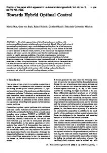
Figure 1: The 2-stage serial inventory/production system of Example 1. stockpoint 1 at the end of a period. So, we pretend that in each stage the value of a product changes at the end of the stage only, i.e., when the product enters the stockpoint at the end of the stage. We assume that we have nonnegative added value per stage, i.e., that H1 ≥ H2 ≥ . . . ≥ HN ≥ 0. For notational convenience, HN +1 := 0. • hn , n = 1, . . . , N : The additional inventory holding cost parameters; hn := Hn −Hn+1 for n = N, . . . , 1. Notice that hn ≥ 0 for all n = 1, . . . , N . • p: Penalty cost parameter. A cost p is charged per unit of backlog at stockpoint 1 at the end of a period. We assume that p > 0. Further notation will be introduced during the analysis as needed. Example 1 During this paper we use a serial system consisting of N = 2 stages, with leadtimes l1 = l2 = 1 and reorder intervals R1 = 2 and R2 = 4, as an illustrative example. This implies that L3 = 0, L2 = 1, L1 = 2, r2 = 1, r1 = 2, r0 = 2, T2 = {0, 4, 8, . . .}, T1 = {1, 3, 5, . . .}. The other input variables are specified when needed. See Figures 1 and 2 for a visualization of the input variables for our example and the time epochs at which orders are placed by stages 1 and 2.

2.3

Objective Function and Echelon Costs

Let Π denote the set of all feasible ordering policies, and let G(π) denote the average costs of ordering policy π for all π ∈ Π. The objective is to find an ordering policy under which the average costs per period are

8

t0∈T2

t0+1

t0+2

t0+3

2

t0+4

t0+5

2 1

1

1 2: order by stage 2 1: order by stage 1

Figure 2: Timing of orders placed by stages 1 and 2 for the system of Example 1. minimized, or, equivalently, to solve: (P ) :

Min

G(π)

s.t.

π ∈ Π.

Here, the average costs consist of inventory holding costs and penalty costs. In Section 4 we will show how the optimal ordering policy can also be found when the objective is to minimize the average inventory holding costs subject to a γ-service level constraint. Before we start with the analysis we have to introduce the concepts echelon stock and echelon inventory position, as well as some relevant cost functions. These are all standard in multi-echelon inventory theory, so we just summarize them here. For an explanation in greater depth, the reader is referred to Zipkin (2000, p. 120-124). The portion of our serial supply chain from the most downstream stockpoint 1 up to any other stockpoint is called an echelon. Echelons are numbered according to the highest stockpoint in that echelon. The echelon stock, or echelon inventory level, of a given echelon n denotes all physical stock at stockpoint n plus all materials in transit to or on hand at any stockpoint downstream, minus a possible backlog at stockpoint 1. The echelon inventory position of an echelon n is defined as its echelon stock plus all materials which are in transit to stockpoint n. As we have centralized control, we may assume w.l.o.g. that a stockpoint never orders more than what is available at the next upstream stockpoint (cf. Chen and Zheng, 1994). Hence, our definition of echelon inventory position is equivalent to defining the echelon inventory position as the echelon stock plus all materials which are on order. The echelon stock and echelon inventory position of echelon n 9

are also called echelon stock n and echelon inventory position n, respectively. We now define so-called costs attached per echelon. Let xn denote echelon stock n at the end of a period. Notice that, by the above definitions, it holds that xn ≥ xn−1 for n = 2, . . . , N . Therefore we find that the total costs at the end of the period under consideration are equal to N X

− Hn (xn − xn−1 ) + H1 x+ 1 + px1

n=2

= HN xN +

N −1 X

(Hn − Hn+1 )xn + (p + H1 )x− 1

n=1

=

N X

hn xn + (p + H1 )x− 1 ,

n=1

where x+ = max{0, x} and x− = max{0, −x} = −min{0, x} for any x ∈ R. This formula shows that the costs may be written as a sum of cost terms per echelon. The costs hn xn are the costs attached to echelon n (or the echelon n costs), n = 2, . . . , N , and the costs h1 x1 + (p + H1 )x− 1 are the costs attached to echelon 1. Notice that the terms hn xn always appear, independent of the sign of xn . Notationally, for each n = 1, . . . , N and t ∈ N0 , we let ILt,n and IPt,n denote echelon stock n (= echelon inventory level n) and echelon inventory position n at the beginning of period t (just before the demand occurs), and we let Ct,n denote the costs attached to echelon n at the end of period t.

3

Analysis

We first show the relationship between, and direct impact of, ordering decisions of different stages, in Subsection 3.1. This constitutes the basis for the analysis of basestock policies and the derivation of an optimal policy, in Subsections 3.2 and 3.3, respectively. In Subsection 3.4, we describe additional results that follow directly from the main results. Finally, an exact solution procedure for the case with mixed Erlang demands is described in Subsection 3.5.

3.1

Setup of the Analysis

In this subsection, we describe the connection between ordering decisions at different stages and which costs they affect.

10

Let t0 be a period in which stage N may place an order; i.e., t0 ∈ TN . By this order, IPt0 ,N is increased to a certain level z. We say that this order starts a whole order cycle in the chain; the ordering decision for stage N in period t0 affects a whole tree of decisions. First, the decision directly affects the ordering by stage N − 1 in the periods τk := t0 + lN + (k − 1)RN −1 , with k = 1, . . . , rN −1 , by which echelon inventory level ILN −1 is increased. Next, each of the ordering decisions for stage N − 1 directly affects the ordering by stage N − 2 in the periods τk + lN −1 + (m − 1)RN −2 , with m = 1, . . . , rN −2 ; and so on. To denote the whole tree of decisions, we introduce the following set of vectors, which has a direct correspondence with the decisions in the order cycle: A

def

=

+1 {(a0 , a1 , . . . , aN ) ∈ NN | ai = 0 for 0 ≤ i ≤ k − 1, where k ∈ {0, . . . , N }, 0

and ai ∈ {1, . . . , ri } for k ≤ i ≤ N } . In addition, for each a ∈ A, we define lev(a) as the index of the first nonzero component of a, i.e., def

lev(a) = min{i|ai > 0} . The vector (0, . . . , 0, 1) is the only vector in A with lev(a) = N . This vector is used as the label for the ordering decision for echelon inventory position N at the beginning of period t0 . Next, the vectors (0, . . . , 0, k, 1), k = 1, . . . , rN −1 (each with level N − 1) are used to denote the ordering decisions for stage N − 1 in the periods t0 + lN + (k − 1)RN −1 ; etcetera. Define def

An = {a ∈ A|lev(a) = n} ,

n = 0, . . . , N.

Thus the vectors a ∈ An , n = 1, . . . , N , denote the decisions at level n in the order cycle, with each vector corresponding to a decision epoch in a specific way. Specifically, vector a ∈ An , n ≥ 1, denotes the ordering def

decision for stage n at the beginning of period ta = t0 + Ln+1 +

PN

i=n (ai − 1)Ri .

The remaining elements of

A, i.e. the vectors a ∈ A0 , are used to label the relevant backlogs as seen by the customers. Vector a ∈ A0 def

is the label for the backlog at stage 1 at the end of period ta = t0 + L1 +

PN

i=0 (ai

− 1)Ri . Finally, for

each a ∈ A \ {(0, . . . , 0, 1)}, we define par(a) as the parent of a, obtained by replacing the first non-zero component of a by a zero. For each a ∈ A \ A0 , the vectors a ˜ ∈ A for which par(˜ a) = a are called the children of a. For all a ∈ An , n ≥ 2, decision a directly affects the decisions a ˜ ∈ An−1 for which par(˜ a) = a. For all a ∈ A1 , decision a directly affects the backlogs a ˜ ∈ A0 for which par(˜ a) = a. 11

Example 1 (continued) For our 2-stage example system, we have: A = {(0, 0, 1), (0, 1, 1), (0, 2, 1), (1, 1, 1), (2, 1, 1), (1, 2, 1), (2, 2, 1)} , lev((0, 0, 1)) = 2 , lev((0, 1, 1)) = lev((0, 2, 1)) = 1 , lev((1, 1, 1)) = lev((2, 1, 1)) = lev((1, 2, 1)) = lev((2, 2, 1)) = 0 , A2 = {(0, 0, 1)} , A1 = {(0, 1, 1), (0, 2, 1)} , A0 = {(1, 1, 1), (2, 1, 1), (1, 2, 1), (2, 2, 1)} , t(0,0,1) = t0 , t(0,1,1) = t0 + 1 , t(0,2,1) = t0 + 3 , t(1,1,1) = t0 + 2 , t(2,1,1) = t0 + 3 , t(1,2,1) = t0 + 4 , t(2,2,1) = t0 + 5 , where t0 ∈ T2 , par((0, 1, 1)) = par((0, 2, 1)) = (0, 0, 1) , par((1, 1, 1)) = par((2, 1, 1)) = (0, 1, 1) , par((1, 2, 1)) = par((2, 2, 1)) = (0, 2, 1) . Here, e.g., the vector (0, 2, 1) denotes the ordering decision taken at stage 1 at time t0 + 3, where t0 ∈ T2 . This decision is directly affected by the parent decision (0, 0, 1). The vector (2, 2, 1) is the label for the backlog at the end of period t0 + 5. See Figure 3.

We now describe which costs are directly affected by the decisions a ∈ A \ A0 , and, while doing that, we also give a more detailed description of the relationship between these decisions a ∈ A \ A0 ,: • Decision a = (0, . . . , 0, 1): This decision concerns the decision at the beginning of period t0 with respect to the order placed by stage N at the external supplier. Suppose that this order is such that the echelon inventory position IPt0 ,N becomes equal to some level z(0,...,0,1) . First of all, this decision directly affects the echelon N costs at the end of the periods t0 + lN + k, k = 0, . . . , RN − 1. The expected values of these costs are equal to E{Ct0 +lN +k,N |IPt0 ,N = z(0,...,0,1) }

=

E{hN (z(0,...,0,1) − Dt0 ,t0 +lN +k )}

=

hN (z(0,...,0,1) − (lN + k + 1)µ) ,

and for the sum we find RX N −1

E{Ct0 +lN +k,N |IPt0 ,N = z(0,...,0,1) }

k=0

h = RN hN ∗ z(0,...,0,1) i 1 −(lN + (RN + 1))µ . 2

12

(1)

Second, decision (0, . . . , 0, 1) affects the decisions a ∈ AN −1 . At the beginning of period τk = t0 + lN + (k − 1)RN −1 , k = 1, . . . , rN −1 , echelon stock N becomes equal to ILτk ,N = z(0,...,0,1) − Dt0 ,τk −1 , and this limits the level to which IPτk ,N −1 can be increased at the beginning of that period τk . These decisions at level N − 1 are the next decisions to consider. • Decisions a ∈ An , for n = N − 1, . . . , 2 (this range of values for n is empty when N = 2): Let n ∈ {2, . . . , N − 1} and a ∈ An . Decision a concerns the decision with respect to the order placed by stage n at the beginning of period ta = t0 + Ln+1 +

PN

i=n (ai − 1)Ri .

Suppose that by this order IPta ,n

becomes equal to some level za . First of all, this decision directly affects the echelon n costs at the end of the periods ta + ln + k, k = 0, . . . , Rn − 1. The expected values of these costs are equal to E{Cta +ln +k,n |IPta ,n = za } = E{hn (za − Dta ,ta +ln +k )} = hn (za − (ln + k + 1)µ) , and for the sum we find RX n −1

E{Cta +ln +k,n |IPta ,n = za }

=

k=0

h i 1 Rn hn za − (ln + (Rn + 1))µ . 2

(2)

Second, decision a affects the decisions a ˜ ∈ An−1 for which par(˜ a) = a. At the beginning of period τm := ta +ln +(m−1)Rn−1 , m = 1, . . . , rn−1 , echelon stock n becomes equal to ILτm ,n = za −Dta ,τm −1 , and this limits the level to which IPτm ,n−1 can be increased at the beginning of period τm . • Decisions a ∈ A1 : Let a ∈ A1 . Decision a concerns the decision with respect to the order placed by stage 1 at the beginning of period ta = t0 + L2 +

PN

i=1 (ai

− 1)Ri . Suppose that by this order IPta ,1

becomes equal to some level za . This decision directly affects the echelon 1 costs at the end of the periods ta + l1 + k, k = 0, . . . , R1 − 1. The expected values of these costs are equal to E{Cta +l1 +k,1 |IPta ,1 = za }

=

E{h1 (za − Dta ,ta +l1 +k ) + (p + H1 )(Dta ,ta +l1 +k − za )+ }

=

h1 (za − (l1 + k + 1)µ) + (p + H1 )E{(Dta ,ta +l1 +k − za )+ } .

13

Start of an ordering cycle

t0

Decision (0,0,1): IPt0,2 is increased up to z(0,0,1) Costs Ct0+k,2 , k =1,2,3,4

Start of next ordering cycle

t0+1

Costs: Ct0+1,2

t0+2

Costs: Ct0+2,2 Ct0+2,1

Decision (0,1,1): IPt0+1,1 is increased up to z(0,1,1) (≤ z(0,0,1) −Dt0, t0 ) Costs Ct0+2,1 and Ct0+3,1

t0+3

t0+4

Costs: Ct0+3,2 Ct0+3,1

t0+5

Costs: Ct0+4,2 Ct0+4,1

Costs: Ct0+5,1

Decision (0,2,1): IPt0+3,1 is increased up to z(0,2,1) (≤ z(0,0,1) −Dt0, t0+2 ) Costs Ct0+4,1 and Ct0+5,1

Figure 3: The relationship between and the consequences of the decisions a ∈ A \ A0 for the system of Example 1. The sum of these expected costs equals RX 1 −1

E{Cta +l1 +k,1 |IPta ,1 = za }

=

k=0

h i 1 R1 h1 za − (l1 + (R1 + 1))µ 2 +(p + H1 )

RX 1 −1

E{(Dta ,ta +l1 +k − za )+ } .

(3)

k=0

Figure 3 illustrates the way in which the above decisions affect each other and which costs are determined by them for Example 1. −1 In the description above, we have explicitly described for each decision a ∈ ∪N n=1 An how the level za to

which IPta ,lev(a) is increased, is bounded from above. We will need this in the analysis below. Obviously, for −1 each decision a ∈ ∪N n=1 An , it also holds that the level za to which IPta ,lev(a) is increased, is bounded from

below (by the level that one already has for echelon inventory position lev(a) just before the new order is placed). In the analysis below, this is taken into account too. But, for the analysis the bounding from below will appear to be less important. 14

The tree of decisions a ∈ A \ A0 starts with decision (0, . . . , 0, 1) taken in a period t0 ∈ TN . It determines the costs Ct0 over the corresponding cycle: def

Ct0 =

N RX N −1 X

Ct0 +Ln +k,n .

n=1 k=0

These costs are defined for each period t0 ∈ TN , and we call them the total costs attached to cycle t0 . Notice that Ct0 contains costs over different shifted time intervals for different echelons. It is easily verified that Ct0 also may be written as Ct0 =

N X RX n −1 X

Cta +ln +k,n .

n=1 a∈An k=0

Example 1 (continued) Let us continue with the illustrative example in order to explain the expressions for Ct0 . Then for each t0 ∈ T2 : Ct0

=

(Ct0 +1,2 + Ct0 +2,2 + Ct0 +3,2 + Ct0 +4,2 ) +(Ct0 +2,1 + Ct0 +3,1 ) + (Ct0 +4,1 + Ct0 +5,1 )

=

2 X RX n −1 X

Cta +ln +k,n .

n=1 a∈An k=0

For each positive recurrent policy π ∈ Π, the average costs are equal to the average value of the costs Ct0 over all cycles t0 ∈ TN divided by the cycle length RN : G(π)

1 = lim E T →∞ T

(T −1 N XX

) Ct,n

t=0 n=1

1 = lim E k→∞ kRN

(kR −1 N N X X t=0

) Ct,n

n=1

  +Ln −1 N LX N kRNX n −1 k−1  X X X 1 = lim E CjRN + Ct,n − Ct,n  k→∞ kRN  n=1 t=0 n=1 j=0 t=kRN

=

lim

k→∞

1 kRN

k−1 X

ECjRN .

(4)

j=0

The above expression requires that the expectations exist and be finite. While this need not be true for general inventory policies (in particular those that do not order sufficiently to satisfy demand), any policy that is positive recurrent will meet this requirement. The class we consider below, basestock policies, are well known to be positive recurrent.

15

3.2

Basestock Policies

A relevant class of ordering policies is constituted by the class of basestock policies. A basestock policy is denoted by a tuple (y1 , . . . , yN ), where yn ∈ R denotes the desired order-up-to level for the echelon inventory position n. Under basestock policy (y1 , . . . , yN ), the ordering decisions are taken as follows: at the beginning of each period t ∈ TN , echelon inventory position N is increased to yN . For each n = N − 1, . . . , 1, at the beginning of each period t ∈ Tn , echelon inventory position n is increased to the minimum of yn and the actual echelon stock of echelon n + 1 (the start up phenomena, occurring in case the initial echelon inventory positions are larger than the desired levels, are ignored, since the long run average costs are not affected by these). Notice that we do not require that the basestock levels be nondecreasing. The average costs for a basestock policy (y1 , . . . , yN ) are denoted by G(y1 , . . . , yN ). It is easily seen that G(y1 , . . . , yN ) = =

1 ECt0 RN Rn −1 N ¯ 1 nX X X ¯ E Cta +ln +k,n ¯z(0,...,0,1) = yN , RN n=1 a∈An k=0

o za = min{ILta ,n+1 , yn } for all n = N − 1, . . . , 1 and a ∈ An ,

(5)

where the tree of decisions a ∈ A \ A0 starts with decision (0, . . . , 0, 1) at the beginning of some period t(0,...,0,1) = t0 ∈ TN (as described in the previous subsection). We now analyze the sums

PRn −1 k=0

Cta +ln +k,n for n = N, . . . , 1 and a ∈ An , referring to formulae (1)-

(3). The term for n = N and a = (0, . . . , 0, 1) is the simplest one. The expected value of the costs PRN −1 k=0

Cta +lN +k,N equals (cf. (1)) RX N −1 k=0

Next, we consider

PRn −1 k=0

h i 1 ECta +lN +k,N = RN hN yN − (lN + (RN + 1))µ . 2

Cta +ln +k,n for n = N − 1 and a ∈ AN −1 . The expected value of this sum is equal

to (cf. (2)) RN −1 −1

X

k=0

i h 1 ECta +lN −1 +k,N −1 = RN −1 hN −1 E{za } − (lN −1 + (RN −1 + 1)µ , 2

with za = min{yN − Dt0 ,ta −1 , yN −1 }. This holds if N ≥ 3; below we describe the formulae for the general case with N ≥ 2. The level za denotes the actual level to which IPta ,N −1 is increased. The difference between this and the desired level yN −1 is called the shortfall, which can also be seen as a backlog at 16

stage N (it would be the backlog at stage N if stage N − 1 would order such that IPta ,N −1 is increased up to yN −1 , without taking into account how much is available at stage N ). We denote this shortfall by Ba = yN −1 − za = yN −1 − min{yN − Dt0 ,ta −1 , yN −1 } = (Dt0 ,ta −1 − (yN − yN −1 ))+ . (Notice that this shortfall is 0 if and only if yN ≥ yN −1 and Dt0 ,ta −1 ≤ yN − yN −1 ; if yN < yN −1 , then this shortfall is positive by definition.) We now find that RN −1 −1

X

k=0

h i 1 ECta +lN −1 +k,N −1 = RN −1 hN −1 yN −1 − (lN −1 + (RN −1 + 1)µ − EBa . 2

A similar expression holds for the sums

PRn −1 k=0

Cta +ln +k,n with n ≤ N − 2 and a ∈ An .

To find the general expressions for the expected values of the sums

PRn −1 k=0

Cta +ln +k,n , for the general

case with N ≥ 2, we define Ba

= 0 for a = (0, . . . , 0, 1),

(6)

Ba

=

(Bpar(a) + Dtpar(a) ,ta −1 − (yn+1 − yn ))+ for all n = N − 1, . . . , 1, a ∈ An ,

(7)

Ba

=

(Bpar(a) + Dtpar(a) ,ta − y1 )+ for all a ∈ A0 .

(8)

For each a ∈ A\A0 , Ba denotes the shortfall when decision a is taken, i.e., the shortfall at stage lev(a)+1 (read external supplier when lev(a) = N ) at the beginning of period ta . For each a ∈ A0 , the random variable Ba denotes the backlog at stage 1 at the end of period ta . Then, using (2) and (3), it can be shown that RX n −1

ECta +ln +k,n

=

k=0 RX 1 −1

ECta +l1 +k,1

=

k=0

h i 1 Rn hn yn − (ln + (Rn + 1))µ − EBa , n = N, . . . , 2, a ∈ An , 2 h i 1 R1 h1 y1 − (l1 + (R1 + 1))µ − EBa 2 X +(p + H1 ) EBa˜ , a ∈ A1 . a ˜∈A0 ,par(˜ a)=a

By substitution of these formulae into (5), we obtain the following theorem. Theorem 2 The average costs of a basestock policy (y1 , . . . , yN ), with yn ∈ R for all n = 1, . . . , N , are equal to G(y1 , . . . , yN )

=

n o Rn X 1 hn yn − (ln + (Rn + 1))µ − EBa 2 RN n=1 a∈An 1 X +(p + H1 ) EBa , RN N X

a∈A0

where the random variables Ba are given by (6)-(8). 17

Proof : Starting with the substitution of the expressions given just before the theorem into equation (5), we obtain: G(y1 , . . . , yN )

=

N h i 1 1 hX X Rn hn yn − (ln + (Rn + 1))µ − EBa RN n=2 2 a∈An h i X n 1 R1 h1 y1 − (l1 + (R1 + 1))µ − EBa + 2 a∈A1 oi X +(p + H1 ) EBa˜ a ˜∈A0 ,par(˜ a)=a

X Rn h = hn yn − (ln + RN n=1 a∈An 1 X +(p + H1 ) RN N X

i 1 (Rn + 1))µ − EBa 2 X EBa˜

a∈A1 a ˜∈A0 ,par(˜ a)=a

o n 1 Rn X = EBa hn yn − (ln + (Rn + 1))µ − 2 RN n=1 a∈An 1 X +(p + H1 ) EBa , RN N X

a∈A0

where in the last step we use that the number of elements of An is equal to |An | =

N Y

ri =

i=n

RN . Rn

Note that as the EBa depend on a, we cannot make this substitution for the remaining sums

P a∈An

EBa in

the last expression.

Theorem 2 gives a very simple expression for the average costs, subject to the evaluation of the average shortfalls/backlogs EBa , a ∈ A. This idea will be important in Subsection 3.5

Example 1 (continued) For our illustrative example, we find that the average costs of a basestock policy (y1 , y2 ), y1 , y2 ∈ R, are equal to G(y1 , y2 )

= h2 {y2 − 72 µ} + h1 {y1 − 52 µ − 21 (EB(0,1,1) + EB(0,2,1) )} +(p + H1 ) · 14 (EB(1,1,1) + EB(2,1,1) + EB(1,2,1) + EB(2,2,1) ) ,

18

(9)

where B(0,1,1) = (Dt0 ,t0 − (y2 − y1 ))+ , B(0,2,1) = (Dt0 ,t0 +2 − (y2 − y1 ))+ , B(1,1,1) = (B(0,1,1) + Dt0 +1,t0 +2 − y1 )+ , B(2,1,1) = (B(0,1,1) + Dt0 +1,t0 +3 − y1 )+ , B(1,2,1) = (B(0,2,1) + Dt0 +3,t0 +4 − y1 )+ , B(2,2,1) = (B(0,2,1) + Dt0 +3,t0 +5 − y1 )+ .

For the sake of the analysis below, we now introduce cost functions Gn (y1 , . . . , yn ), with n = 1, . . . , N , and yi ∈ R for all i = 1, . . . , n. The function Gn (y1 , . . . , yn ) is defined as the average costs attached to the echelons 1, . . . , n when each of the stages 1, . . . , n applies a basestock policy with basestock level yi and when stage n + 1 can always deliver. Obviously, GN (y1 , . . . , yN ) = G(y1 , . . . , yN ). For the functions Gn (y1 , . . . , yn ) we can derive expressions similar to G(y1 , . . . , yN ). We first define A(n)

def

=

{(a0 , a1 , . . . , an ) ∈ Nn+1 |ai = 0 for 0 ≤ i ≤ k − 1, where k ∈ {0, . . . , n}, 0 ai ∈ {1, . . . , ri } for k ≤ i ≤ n − 1, an = 1} , (n)

and then define lev(a), Ai

and par(a) respective to A(n) in an analogous manner as we did for the set A.

Then it is easily verified that (cf. Equation (5)) Gn (y1 , . . . , yn ) =

Ri −1 n ¯ 1 nX X X ¯ E Cta +li +k,i ¯z(0,...,0,1) = yn , Rn (n) i=1 a∈Ai

k=0

(n)

za = min{ILta ,i+1 , yi } for all 1 ≤ i ≤ n − 1 and a ∈ Ai (n)

where the tree of decisions a ∈ A(n) \ A0

def

n X

lj +

j=i+1

n X

(aj − 1)Rj ,

(n)

i = 0, . . . , n, a ∈ Ai .

j=i

Next, along the same lines as Theorem 2, we find the following result. Lemma 3 For n = 1, . . . , N , and yi ∈ R for all i = 1, . . . , n, Gn (y1 , . . . , yn )

=

(10)

starts with decision (0, . . . , 0, 1) at the beginning of some period

t(0,...,0,1) = t0 ∈ Tn , and ta = t0 +

o ,

n o Ri X 1 hi yi − (li + (Ri + 1))µ − EBa(n) 2 Rn (n) i=1

n X

+(p + H1 )

1 Rn

X (n) a∈A0

19

a∈Ai

EBa(n) ,

(n)

where the random variables Ba

are defined by

Ba(n)

= 0 for a = (0, . . . , 0, 1),

Ba(n)

= (Bpar(a) + Dtpar(a) ,ta −1 − (yi+1 − yi ))+ for all 1 ≤ i ≤ n − 1, a ∈ Ai ,

Ba(n)

= (Bpar(a) + Dtpar(a) ,ta − y1 )+ for all a ∈ A0 .

(N )

Notice that Ba

(n)

(n)

(n)

(n)

= Ba for all a ∈ A(N ) = A. For n = 1, . . . , N − 1 (the formulation that follows also holds (n)

for n = N ), the Ba

are related to the Ba as follows. Let n ∈ {1, . . . , N − 1} and let a ˜ ∈ An . Then d

Ba(n) = (B(a0 ,...,an−1 ,˜an ,...,˜aN ) |Ba˜ = 0) d

for all a ∈ A(n) ,

(n)

where = denotes equality in distribution. In other words, Ba

is equal in distribution to the shortfall of any

full N -vector on the same decision epoch under the condition that there is no shortfall upstream of stage n in the N -vector. (k)

Similarly, the Ba

(n)

are related to the Ba

for some k < n as follows. Let k, n ∈ {1, . . . , N } with k < n

(n)

and let a ˜ ∈ Ak . Then d

(n)

(n)

Ba(k) = (B(a0 ,...,ak−1 ,˜ak ,...,˜an ) |Ba˜

for all a ∈ A(k) .

= 0)

(11)

For each of the functions Gn (y1 , . . . , yn ), we also need the partial derivative with respect to the last component yn . Hence, for n = 1, . . . , N , we define def

gn (y1 , . . . , yn ) =

δ {Gn (y1 , . . . , yn )} , yi ∈ R for all i = 1, . . . , n. δyn

For the partial derivatives, the following result holds. Lemma 4 For n = 1, . . . , N , and yi ∈ R for all i = 1, . . . , n, gn (y1 , . . . , yn )

=

n X

hi − (p + H1 )

i=1

−

n−1 X i=1

1 X P{Ba(n) > 0} Rn (n) a∈A0

Ri Rn

X

P{Ba(n) = 0}gi (y1 , . . . , yi )

(n)

a∈Ai

(with the convention that the last sum on the righthand side is equal to 0 when n = 1). The proof of this lemma is given in the appendix. 20

3.3

Derivation of an Optimal Policy

Consider again the tree of decisions a ∈ A \ A0 which starts with decision (0, . . . , 0, 1) in some period t0 ∈ TN ; see the description in Subsection 3.1. We first consider how these decisions can be taken such that the expected total costs attached to cycle t0 (= ECt0 ) are minimized. Each decision a ∈ An , with n = 1, . . . , N , is described by the level za , to which echelon inventory position n is increased at the beginning of period ta . The choice for the level za is limited from above by what is available at the next upstream stage and from below by the value of echelon inventory position n just before the order is placed. For the moment, we neglect the bounding from below, and we consider the following relaxed problem (RP (t0 )): Min ECt0 =

N X RX n −1 X

ECta +ln +k,n

n=1 a∈An k=0

s.t. RX 1 −1 k=0

h i 1 ECta +l1 +k,1 = R1 h1 za − (l1 + (R1 + 1))µ 2 +(p + H1 )

RX 1 −1

E{(Dta ,ta +l1 +k − za )+ } , a ∈ A1 ,

k=0 RX n −1 k=0

h i 1 ECta +ln +k,n = Rn hn za − (ln + (Rn + 1))µ , n = 2, . . . , N, a ∈ An , 2

za ≤ ILta ,n+1 , n = 1, . . . , N − 1, a ∈ An , ILta ,n+1 = zpar(a) − Dtpar(a) ,ta −1 , n = 1, . . . , N − 1, a ∈ An . The solution of this N -stage stochastic programming problem follows from the following lemma. Lemma 5 For n equal to successively 1, . . . , N : (i) If n = 1, then g1 (y1 )

= h1 − (p + H1 )

1 X P{Ba(1) > 0} , R1 (1)

y1 ∈ R,

a∈A0

with Ba(1)

(1)

= (Dtpar(a) ,ta − y1 )+ for all a ∈ A0 .

If n ∈ {2, . . . , N }, then gn (S1 , . . . , Sn−1 , yn ) =

n X

hi − (p + H1 )

i=1

1 X P{Ba(n) > 0} , yn ∈ R, Rn (n) a∈A0

21

with Ba(n)

= 0

Ba(n)

= (Bpar(a) + Dtpar(a) ,ta −1 − (yn − Sn−1 ))+ for all a ∈ An−1 ,

Ba(n)

= (Bpar(a) + Dtpar(a) ,ta −1 − (Si+1 − Si ))+ for all i = n − 2, . . . , 1, a ∈ Ai ,

Ba(n)

= (Bpar(a) + Dtpar(a) ,ta − S1 )+ for all a ∈ A0 .

for a = (0, . . . , 0, 1), (n)

(n)

(n)

(n)

(n)

(n)

(if one or more of the Si are equal to infinity, then in these formulae the Si have to be read as if they are equal to a very large finite constant). (ii) gn (S1 , . . . , Sn−1 , yn ) is continuous and nondecreasing as a function of yn . In particular, gn (S1 , . . . , Sn−1 , yn ) = −(p + Hn+1 ) (< 0) for all yn ≤ 0 and gn (S1 , . . . , Sn−1 , yn ) ↑ hn (≥ 0) as yn → ∞. (iii) Gn (S1 , . . . , Sn−1 , yn ) is convex as a function of yn . (iv) Let Sn (∈ R ∪ {∞}) be chosen such that def

Sn = argminyn ∈R Gn (S1 , . . . , Sn−1 , yn ) Then Sn is such that gn (S1 , . . . , Sn−1 , Sn ) = 0. In particular, Sn is positive and finite if hn > 0; Sn = ∞ if hn = 0 and F has infinite support; Sn is positive and may be finite as well as infinite if hn = 0 and F has finite support. (v) For the problem (RP(t0 )), it is optimal to choose each of the levels za , a ∈ An , equal to Sn , or as high as possible if this level can not be reached. The proof of this lemma is given in the appendix. By, Lemma 5, basestock policy (S1 , . . . , SN ) is optimal for the relaxed problem RP(t0 ). The problem was obtained by neglecting the bounding from below when placing orders. However, the optimality of basestock policy (S1 , . . . , SN ) holds for each cycle t0 ∈ TN . If this basestock policy is used in all cycles, then these lower bounds at most constitute a limitation during a transient period (when the echelon inventory positions may be above the Sn , and nothing should be ordered). Hence, in the long run basestock policy (S1 , . . . , SN ) is also feasible for the un-relaxed version of RP(t0 ), and hence also optimal for this problem. Thus basestock policy (S1 , . . . , SN ) is also optimal for problem (P). 22

Theorem 6 Basestock policy (S1 , . . . , SN ) with the Sn as defined in Lemma 5 is optimal for problem (P). The optimal basestock levels (S1 , . . . , SN ) satisfy the Newsboy-type characterizations listed in the following corollary, which immediately follows from the parts (i)-(iv) of Lemma 5. Corollary 7 The optimal basestock levels S1 , . . . , SN are such that for each n = 1, . . . , N , 1 X p + Hn+1 P{Ba(n) = 0} = , Rn p + H1 (n) a∈A0

with Ba(n)

=

0

Ba(n)

=

(Bpar(a) + Dtpar(a) ,ta −1 − (Si+1 − Si ))+

Ba(n)

=

(Bpar(a) + Dtpar(a) ,ta − S1 )+

for a = (0, . . . , 0, 1), (n)

(n)

(n)

for all i = n − 1, . . . , 1, a ∈ Ai , (n)

for all a ∈ A0 .

This corollary says that, when Sn is determined, it is imagined that stage n + 1 can always deliver (i.e., the analysis is limited to the chain consisting of the stages n, . . . , 1) and the value for Sn is chosen such that the average probability for a nonnegative stock at the most downstream stage 1 is equal to

p+Hn+1 p+H1

(notice

that the non-stockout probability in any period has a cyclic pattern).

Example 1 (continued) For our illustrative example, an optimal policy (S1 , S2 ) is as follows. By Corollary 7 and some algebra, we find that basestock level S1 satisfies o p+H 1n 2 P{Dt0 ,t0 +1 ≤ S1 } + P{Dt0 ,t0 +2 ≤ S1 } = , 2 p + H1

(12)

where t0 is an arbitrary period in which stage 1 orders (i.e., t0 ∈ T1 ). So, under the assumption that stage 1 never experiences a shortage at stage 2, S1 is such that the average non-stockout probability per cycle of 2 periods is equal to

p+H2 p+H1 .

Basestock level S2 satisfies

1n P{(Dt0 ,t0 − (S2 − S1 ))+ + Dt0 +1,t0 +2 ≤ S1 } 4 + P{(Dt0 ,t0 − (S2 − S1 ))+ + Dt0 +1,t0 +3 ≤ S1 } + P{(Dt0 ,t0 +2 − (S2 − S1 ))+ + Dt0 +3,t0 +4 ≤ S1 } o + P{(Dt0 ,t0 +2 − (S2 − S1 ))+ + Dt0 +3,t0 +5 ≤ S1 } = 23

p , p + H1

(13)

where t0 is an arbitrary period in which stage 2 orders (i.e., t0 ∈ T2 ). S2 is such that the average non-stockout probability per cycle of 4 periods is equal to

p p+H1 .

Note that since the demand distribution F is continuous,

(S1 , S2 ) can be chosen to satisfy these equations.

3.4

Additional Results

The following corollary says that it is sufficient to hold stocks at the end of the most downstream stage 1 and in front of stages where value is added to the product; i.e., it is not necessary to hold stock in front of stages n (< N ) with hn = 0. Corollary 8 There exists an optimal basestock policy under which no safety stocks are held in front of stages where zero value is added. Proof : Suppose that hn = 0 for some stage n = 1, . . . , N − 1. Then, by part (iv) of Lemma 5, Sn may be chosen equal to Sn = ∞. This implies that in each period all goods arriving in stockpoint n + 1 are immediately forwarded to stockpoint n. This means that there is never stock present in stockpoint n + 1 at the end of a period.

For the basestock policies we have not assumed that they have nondecreasing basestock levels. In fact, such an assumption would have complicated our analysis. The following corollary relates a general basestock policy to a basestock policy with nondecreasing basestock levels. def

Corollary 9 Let yn ∈ R for n = 1, . . . , N , and define y˜n = min{yn , . . . , yN } for n = 1, . . . , N . Then G(˜ y1 , . . . , y˜N ) = G(y1 , . . . , yN ). This corollary follows directly from Theorem 2. In fact, it is easily verified that under basestock policy (˜ y1 , . . . , y˜N ) the orders are identical to the orders generated under basestock policy (y1 , . . . , yN ) (at least in the long run; in the first periods of the horizon there may be differences).

24

3.5

Exact Solution Procedure for Mixed Erlang Demands

In general, an optimal basestock policy (S1 , . . . , SN ) and the corresponding average costs can be computed as follows. First, for n = 1, . . . , N , Sn may be computed by the Newsboy-type characterization in Corollary 7, where in each step bisection is applied. Next, the optimal average costs G(S1 , . . . , SN ) follow from Theorem 2. For both, it is required that for a given basestock policy we are able to evaluate the shortfalls/backlogs (n)

Ba

as defined in Corollary 7 and the Ba given by (6)-(8). These shortfalls/backlogs may be determined

recursively after a sufficiently fine discretization of the one-period demand distribution F , although that may be computationally inefficient, in particular as N grows large. We describe an alternative, efficient procedure that is applicable when the one-period demand is a mixture of Erlang distributions with the same scale parameter. This is described below. Modeling demand as a mixture of Erlangs with the same scale parameter is motivated by the fact that this class of distributions is dense in the class of all distributions on [0, ∞). We assume that the one-period demand is simply given as such a distribution. In practice, however, often only the first two moments of the one-period demand are given, and then a two-moment fit may be applied first: a so-called Erlang(k −1, k) distribution can be fitted if the coefficient of variation of the demand is smaller than or equal to 1, and a so-called Erlang(1, k) distribution otherwise. More moments may be fit as desired, yielding a larger mixture. Let us assume that the demand distribution F is a mixture of Erlang distributions with the same scale parameter; i.e., there is a discrete distribution on N, {qk }k∈N , and a λ > 0 such that F (x) =

P∞

k=1 qk Ek,λ (x),

x ∈ R, where Ek,λ denotes the Erlang distribution with k ∈ N phases and scale parameter λ > 0. We describe (n)

the evaluation of the Ba

as defined in Corollary 7, for n ≥ 3. The evaluation for all other cases is similar. (n)

(n)

For a = (0, . . . , 0, 1), which is the only element of An , it is given that Ba

= 0 (which may be seen as (n)

a mixture of Ek,λ with all probability mass in 0. Next, we can determine the Ba (n)

this case, Ba

(n)

for each a ∈ An−1 . In

= (Dtpar(a) ,ta −1 − (Sn − Sn−1 ))+ . The random variable Dtpar(a) ,ta −1 is the (ta − tpar(a) )-fold

convolution of the one-period demand, and thus is also a mixture of Erlang distributions with scale parameter λ. The mixture probabilities are equal to the (ta − tpar(a) )-fold convolution of {qk }k∈N . Next, if Sn > Sn−1 , then we shift the distribution of Dtpar(a) ,ta −1 to the left over a distance Sn − Sn−1 , while the probability mass that would arrive in the negative range is absorbed in 0. By that operation, we obtain the distribution

25

of (Dtpar(a) ,ta −1 − (Sn − Sn−1 ))+ , which is a mixture of Ek,λ distributions with a positive probability mass in 0 (for the computation of the new mixture probabilities, see Scheller-Wolf et al., 2003). If Sn ≤ Sn−1 , then we shift the distribution of Dtpar(a) ,ta −1 to the right over a distance Sn−1 − Sn . Then, the random variable (Dtpar(a) ,ta −1 − (Sn − Sn−1 ))+ consists of a deterministic part plus a mixture of Ek,λ distributions. (n)

Next, the Ba

(n)

(n)

= (Bpar(a) + Dtpar(a) ,ta −1 − (Sn−1 − Sn−2 ))+ for each a ∈ An−2 may be determined, and so (n)

on. The procedure is the same then, except that each time first the convolution of Dtpar(a) ,ta −1 with Bpar(a) has to be determined. This again will be a mixture of Erlang distributions with the same scale parameter λ, possibly plus a deterministic part (see Scheller-Wolf et al., 2003). The reason that the above procedure works is that the class of Erlang distributions with the same scale parameter, with possibly a positive probability mass in 0 or a deterministic part being added, is closed under the shift operation as described above and when convolutions are taken. The above procedure is simpler to implement than the exact procedure described in Van Houtum and Zijm (1997) for the standard Clark-and-Scarf model. Finally, the general class of phase-type distributions is likewise closed under the convolution and shift operation. So, an exact procedure can also be derived for phase-type distributions, although the different steps may become more complicated. If one is satisfied with accurate approximations, then one may use the simple approximate procedure based on two-moment fits as described in Van Houtum and Zijm (1991).

Example 1 (continued) For our illustrative example, we have the formulae (9), (12), and (13) available. Assume that H2 = 0.5, H1 = 1, p = 20 and that one-period demand is exponential with mean µ = 1. Then, by the exact solution procedure, we find unique optimal basestock levels S1 = 6.67 and S2 = 9.90, and optimal costs G(S1 , S2 ) = 5.84. The corresponding computation time on a regular Pentium III PC is negligibly small (only a flash).

26

4

Extensions

4.1

Service Level Problem

We now consider our model with a γ-service level constraint (which is equivalent to an average backlog constraint) instead of penalty costs. The γ-service level is also known as modified fill rate, and is closely related to the regular fill rate. For high service levels (more precisely, as long as any demand is not backordered for more than one period), both measures are identical (see Van Houtum et al., 1996). Let γ0 be the target γ-service level. We assume that the demand distribution F has a compact support. Then an optimal policy is obtained as described below. First, by Theorem 2, we find that the γ-service level of a basestock policy (y1 , . . . , uN ) equals γ(y1 , . . . , yN ) = 1 −

1 1 X EBa , µ RN a∈A0

where the random variables Ba are given by (6)-(8). Second, if for the penalty cost model with a given penalty cost parameter p, the resulting optimal policy (S1 , . . . , SN ) has a γ-service level γ(S1 , . . . , SN ) = γ(p) that is precisely equal γ0 , then (S1 , . . . , SN ) is also optimal for the service level problem with target service level γ0 (see Theorem 1 of Van Houtum and Zijm, 2000). Third, the function γ(p) is nondecreasing as a function of p (see Theorem 2 of Van Houtum and Zijm, 2000). Forth, under the assumption that F has compact support, one can show that the optimal basestock levels S1 , . . . , SN are continuous as a function of p; thus, also γ(p) is continuous as a function of p, and further γ(p) ↑ 1 as p → ∞. The above shows that the service level problem with a given target level γ0 < 1 may be solved by solving the penalty cost problem and tuning the penalty cost parameter p such that the γ-service level γ(p) of the optimal policy equals γ0 . Also, this implies that the class of basestock policies is also optimal for the service level problem with a γ-service level constraint.

4.2

Non-Synchronized Reorder Epochs

We have assumed that the synchronization constraint is satisfied for the reorder epochs Tn of the stages n = 1, . . . , N . If this constraint is not satisfied, then the results still hold but for a system with adapted leadtimes. This is illustrated for the system of Example 1. Assume that for this example system everything 27

is as previously described but stage 1 is now allowed to order at the beginning of the periods 0, 2, 4, . . .; i.e., T1 = {0, 2, 4, . . .} instead of T1 = {1, 3, 5, . . .}. Then each shipment arriving in stockpoint 2 has to wait at least one period before materials may enter stage 1, as if the leadtime for stage 2 equals ˜l2 = 2 instead of l2 = 1. Everything else is the same as in the original system synchronized reorder epochs. Thus all results apply, where in all formulae l2 has to be replaced by ˜l2 .

4.3

Order Frequencies with Non-Integer Ratios

In our model, we also assumed that the reorder intervals satisfy the integer-ratio constraint. If this constraint is not satisfied, then the optimal policy may be a basestock policy with time-dependent basestock levels or possibly even more complicated. Nevertheless, for practical purposes, it may be useful to consider basestock policies only, and to optimize within this class. For the average costs, one then has to look at a cycle with a length equal to the least common multiple of R1 , . . . , RN . For the average costs of a basestock policy, similar formulae will be obtained as in Theorem 2. To find optimal basestock levels, we suggest deriving partial derivatives and to apply a standard procedure for the minimization of a multi-dimensional function.

4.4

Assembly Systems

Assembly systems without periodic batching can be shown to be equivalent to serial systems; see Rosling (1989). This equivalence is built on the property that for a given component it is never optimal to order more than the amount of companion components that will be available at the next assembly point. This property also applies to assembly systems with periodic batching. Thus, each assembly system with periodic batching is equivalent to a serial system with periodic batching. If this equivalent serial system satisfies the synchronization and integer-ratio constraint, then all results of this paper apply again. Otherwise, see Subsections 4.2 and 4.3.

5

Concluding Remarks

We have studied a serial, multi-echelon inventory system with periodic batching. We have been able to generalize many of the results known for the standard Clark-and-Scarf model. In further research, we will 28

consider multi-echelon systems with a divergent structure and periodic batching, which are relevant for production and distribution environments. There we can build on available results for divergent systems without batching; see e.g. Diks and De Kok (1998). Also, we will work on developing appropriate models for the upper decision level of the hierarchical approach as described in the introduction of this paper.

Appendix Proof of Lemma 4 By Lemma 3, for all n = 1, . . . , N and yi ∈ R for i = 1, . . . , n, gn (y1 , . . . , yn ) = hn −

n−1 X

hi

i=1 (n)

noting that Ba

Ri X δ 1 X δ {EBa(n) } + (p + H1 ) {EBa(n) } , Rn δyn Rn δyn (n) (n) a∈Ai

a∈A0

(n)

= 0 for a ∈ An .

For each a = (a0 , a1 , . . . , an ) ∈ A(n) , we define def

pj (a) = (0, . . . , 0, aj , . . . , an )

for j = lev(a), . . . , n.

The vector pj (a) is the unique vector at level j on the path from a to (0, . . . , 0, 1) in the tree constituted by the elements of A(n) , where the tree is rooted at (0, . . . , 0, 1) and edges correspond to parent-child relationships. In particular, plev(a) (a) = a for all a ∈ A(n) , and plev(a)+1 (a) = par(a) for all a ∈ A(n) \ {(0, . . . , 0, 1)}. It is easily verified now that for each a ∈ A(n) \ {(0, . . . , 0, 1)}, δ (n) {EBa(n) } = −P{Bpj (a) > 0 for j = n − 1, . . . , lev(a)}, δyn i.e., in order for an increase in yn to have an effect on the backorder at a given a below the root of the tree, there must be a path of positive backlogs in the tree between the root and a. By substitution of this result in the formula given above for gn (y1 , . . . , yn ), we obtain gn (y1 , . . . , yn )

= hn +

n−1 X i=1

hi

Ri X (n) P{Bpj (a) > 0 for j = n − 1, . . . , i} Rn (n)

− (p + H1 )

a∈Ai

1 X (n) P{Bpj (a) > 0 for j = n − 1, . . . , 0}. Rn (n) a∈A0

29

(14)

For n = 1, formula (14) reads as 1 X P{Ba(1) > 0} . R1 (1)

g1 (y1 ) = h1 − (p + H1 )

a∈A0

This expression is identical to the formula given by Lemma 4. We now show that the formula given by the Lemma 4 is also correct for each n = 2, . . . , N . Consider (n)

Equation (14). For each i = 1, . . . , n − 1 and a ∈ Ai , we find that (n)

P{Bpj (a) > 0 for j = n − 1, . . . , i} (n)

= 1 − P{Bpj (a) = 0 for some j = n − 1, . . . , i} =1−

n−1 X

(n)

(n)

P{Bpk (a) = 0, Bpj (a) > 0 for j = k − 1, . . . , i}

k=i

=1−

n−1 X

(n)

(n)

(n)

P{Bpj (a) > 0 for j = k − 1, . . . , i|Bpk (a) = 0}P{Bpk (a) = 0}

k=i (n)

(n)

(with the convention that P{Bpj (a) > 0 for j = k − 1, . . . , i|Bpk (a) = 0} = 1 when k = i). Similarly, for each (n)

a ∈ A0 , we find (n)

P{Bpj (a) > 0 for j = n − 1, . . . , 0} (n)

= P{Ba(n) > 0} − P{Bpj (a) = 0 for some j = n − 1, . . . , 1, Ba(n) > 0} =

P{Ba(n)

> 0} −

n−1 X

(n)

(n)

P{Bpk (a) = 0, Bpj (a) > 0 for j = k − 1, . . . , 0}

k=1

= P{Ba(n) > 0} −

n−1 X

(n)

(n)

(n)

P{Bpj (a) > 0 for j = k − 1, . . . , 0|Bpk (a) = 0}P{Bpk (a) = 0} .

k=1

30

By substitution of these expressions into Equation (14), we obtain gn (y1 , . . . , yn ) =

hn +

n−1 X

Ri X h 1 Rn (n)

hi

i=1

−

n−1 X

a∈Ai

(n)

(n)

i

(n)

P{Bpj (a) > 0 for j = k − 1, . . . , i|Bpk (a) = 0}P{Bpk (a) = 0}

k=i

− (p + H1 )

1 X h P{Ba(n) > 0} Rn (n) a∈A0

−

n−1 X

(n)

(n)

i

(n)

P{Bpj (a) > 0 for j = k − 1, . . . , 0|Bpk (a) = 0}P{Bpk (a) = 0}

k=1 n X

=

hi − (p + H1 )

i=1

−

1 X P{Ba(n) > 0} Rn (n) a∈A0

n−1 k XX

hi

k=1 i=1

Ri X (n) (n) P{Bpj (a) > 0 for j = k − 1, . . . , i|Bpk (a) = 0} Rn (n) a∈Ai

(n)

P{Bpk (a) = 0} +

n−1 X k=1

(p + H1 ) X

1 Rn (n)

(n)

P{Bpj (a) > 0 for j = k − 1, . . . , 0|Bpk (a) = 0}

(n)

a∈A0

(n)

P{Bpk (a) = 0}.

(15) (k)

By using the relationships, for different values of k, between the sets Ai (k)

Ba

and between the random variables

(cf. (11)), we find for all k = 1, . . . , n − 1 and i = 1, . . . , k, X

(n)

(n)

(n)

P{Bpj (a) > 0 for j = k − 1, . . . , i|Bpk (a) = 0}P{Bpk (a) = 0}

(n)

a∈Ai

= =

X

X

(n) a ˆ∈Ak

(n) a∈Ai ,pk (a)=ˆ a

X

(n)

P{Baˆ

(n)

(n)

P{Bpj (a) > 0 for j = k − 1, . . . , i|Baˆ

= 0}

(n)

X

(n)

= 0}P{Baˆ

= 0}

(k)

P{Bpj (˜a) > 0 for j = k − 1, . . . , i}

(k)

a ˆ∈Ak

a ˜∈Ai (k)

(with the convention that P{Bpj (˜a) > 0 for j = k − 1, . . . , i} = 1 when k = i). Similarly, we find for all k = 1, . . . , n − 1, X

(n)

(n)

(n)

P{Bpj (a) > 0 for j = k − 1, . . . , 0|Bpk (a) = 0}P{Bpk (a) = 0}

(n)

a∈A0

=

X (n)

a ˆ∈Ak

(n)

P{Baˆ

= 0}

X

(k)

P{Bpj (˜a) > 0 for j = k − 1, . . . , 0} .

(k)

a ˜∈A0

31

By substitution of these expressions into Equation (15), and by using (14), we find gn (y1 , . . . , yn ) =

n X

hi − (p + H1 )

i=1

−

n−1 X k=1

a∈A0

k hX Ri X Rk X (n) (k) hi P{Baˆ = 0} P{Bpj (˜a) > 0 for j = k − 1, . . . , i} Rn R k (n) (k) i=1 a ˆ∈Ak

a ˜∈Ai

−(p + H1 )

=

n X

1 X P{Ba(n) > 0} Rn (n)

hi − (p + H1 )

i=1

1 Rk

X

i

(k)

P{Bpj (˜a) > 0 for j = k − 1, . . . , 0}

(k)

a ˜∈A0

n−1 X Rk X 1 X (n) P{Ba(n) > 0} − P{Baˆ = 0}gk (y1 , . . . , yk ) , Rn R n (n) (n) k=1

a∈A0

a ˆ∈Ak

(n)

(again with the convention that P{Bpj (˜a) > 0 for j = k − 1, . . . , i} = 1 when i = k and a ˜ = (0, . . . , 0, 1)). This completes the proof.

Proof of Lemma 5 We prove Lemma 5 by induction to n. Let n = 1. Then, the formula in part (i) is identical to the formula in Lemma 4 with n = 1, and hence correct. From this formula, it immediately follows that g1 (y1 ) is continuous and nondecreasing. In particular, g1 (y1 ) is equal to −(p + H2 ) < 0 for all y1 ≤ 0 and it goes to h1 for y1 → ∞. If the demand distribution (1)

F has finite support, then also the distributions of the Dtpar(a) ,ta , a ∈ A0 , have finite support and the derivative will be equal to h1 for all values larger than or equal to a certain finite point. The behavior of g1 (y1 ) implies that G1 (y1 ) is convex. This completes the proof of part (i)-(iii). Next, S1 is defined as a point where G1 (y1 ) is minimized. If there are multiple points where G1 (y1 ) is minimized, then S1 may be taken equal to any of these points. Obviously, since g1 (y1 ) < 0 for all y1 ≤ 0 and g1 (y1 ) is continuous, we find that S1 > 0. Further, if h1 > 0, then S1 < ∞. If h1 = 0 and the demand distribution F has a finite support, then S1 can be chosen equal to a finite value or equal to S1 = ∞. If h1 = 0 and the demand distribution F has an infinite support, then S1 = ∞. In all these cases, S1 is such that g1 (y1 ) = 0 for y1 = S1 . This proves part (iv). We can now show how the decision a ∈ A1 , i.e., the choices for the za with a ∈ A1 , may be optimized for problem (RP(t0 )). Let a ∈ A1 . Decision a is taken at the beginning of period ta , and the choice for za is bounded from above by ILta ,2 . This decision only affects the costs 32

PR1 −1 k=0

ECta +l1 +k,1 , which, by (10), are

equal to G1 (za ). These costs are minimized by choosing za equal to za = S1 if ILta ,2 ≥ S1 , and equal to za = ILta ,2 if ILta ,2 < S1 . This completes the proof of part (v), and hence also the proof of the complete lemma for n = 1. Let us now suppose that the results above have been proved for all m = 1, . . . , n−1, where n ∈ {2, . . . , N }. We shall prove that then the results also hold for m = n. The derivative of Gn (S1 , . . . , Sn−1 , yn ) as a function of yn is given by (cf. Lemma 4) gn (S1 , . . . , Sn−1 , yn ) =

n X

hi − (p + H1 )

i=1

−

a∈A0

n−1 X i=1

(n)

where the Ba

1 X P{Ba(n) > 0} Rn (n)

Ri X P{Ba(n) = 0}gi (S1 , . . . , Si ) , Rn (n)

yn ∈ R,

a∈Ai

are defined as in part (i) of Lemma 5. By the induction assumption, gi (S1 , . . . , Si ) = 0 for

each i = 1, . . . , n − 1. Hence, all terms in the third sum in the formula for gn (S1 , . . . , Sn−1 , yn ) vanish, and we find the formula given in part (i) of Lemma 5. (n)

It is easily verified that the distribution functions of the Ba , a ∈ A(n) , behave continuously as a function of yn and that they are stochastically decreasing (= non-increasing) as a function of yn . Hence, gn (S1 , . . . , Sn−1 , yn ) is continuous and nondecreasing as a function of yn . In particular, this function appears (n)

to be equal to −(p + Hn+1 ) < 0 for all yn ≤ 0. Note that if yn = 0, then it holds that P{Ba (n)

(n)

all a ∈ A0 . The number of elements of A0

> 0} = 1 for

is equal to r0 r1 · · · rn−1 = Rn . Hence,

n X

N X 1 gn (S1 , . . . , Sn−1 , 0) = hi − (p + H1 ) Rn = −(p + hi ) = −(p + Hn+1 ) < 0 . Rn i=1 i=n+1

Further, gn (S1 , . . . , Sn−1 , yn ) ↑ hn when yn → ∞. To show the latter, we distinguish two cases. The first case is when Si = ∞ for all i = 1, . . . , n − 1. Then, first of all, it must hold that hi = 0 for all (n)

(n)

i = 1, . . . , n − 1 (by the induction assumption). Further, the expressions for the Ba , a ∈ A0 , reduce to

33

(n)

Ba

= (Dt(0,...,0,1) ,ta − yn )+ (take S1 = . . . = Sn−1 = M and let M → ∞): Ba(n)

=

0

Ba(n)

=

(Bpar(a) + Dtpar(a) ,ta −1 − (yn − M ))+

=

Dt(0,...,0,1) ,ta −1 + M − yn

=

(Bpar(a) + Dtpar(a) ,ta −1 − (M − M ))+

=

Dt(0,...,0,1) ,tpar(a) −1 + M − yn + Dtpar(a) ,ta −1

=

Dt(0,...,0,1) ,ta −1 + M − yn

=

(Bpar(a) + Dtpar(a) ,ta − M )+

=

(Dt(0,...,0,1) ,tpar(a) −1 + M − yn + Dtpar(a) ,ta − M )+

=

(Dt(0,...,0,1) ,ta − yn )+

Ba(n)

for a = (0, . . . , 0, 1), (n)

(n)

for all a ∈ An−1 ,

(n)

(n)

for all a ∈ An−2 ,

... Ba(n)

(n)

Hence, if yn → ∞, P{Ba

(n)

(n)

for all a ∈ A0 .

> 0} ↓ 0 for all a ∈ A0 , and thus gn (S1 , . . . , Sn−1 , yn ) →

Pn i=1

hi = hn (as hi = 0

for all i ≤ n − 1). The second case is when there is at least one Si which is finite. Then we define the index k by k := max{i|Si < ∞}. Then, first of all, it must hold that hi = 0 for all i = k + 1, . . . , n − 1 (by the (n)

(n)

induction assumption). Further, the expressions for the Ba , a ∈ ∪ni=k Ai , reduce in a manner similar as above to: (n)

Ba(n) = (Dt(0,...,0,1) ,ta −1 − (yn − Sk ))+ for all a ∈ Ak (notice that this is only a real reduction when k < n − 1). Further, (n)

(n)

Ba(n)

=

(Bpar(a) + Dtpar(a) ,ta −1 − (Si+1 − Si ))+ for all 1 ≤ i ≤ k − 1, a ∈ Ai ,

Ba(n)

=

(Bpar(a) + Dtpar(a) ,ta − S1 )+ for all a ∈ A0 .

(n)

(n)

(n)

(n)

(notice that this is only a real reduction when k < n − 1). Hence, if yn → ∞, then for each a ∈ Ak , Ba (n)

(n)

(k)

(k) becomes equal to 0, and the Ba , a ∈ ∪k−1 , i=0 Ai , become identical to the random variables Ba , a ∈ A

34

given by Ba(k)

=

0 for a = (0, . . . , 0, 1),

Ba(k)

=

(Bpar(a) + Dtpar(a) ,ta −1 − (Si+1 − Si ))+ for all 1 ≤ i ≤ k − 1, a ∈ Ai ,

Ba(k)

=

(Bpar(a) + Dtpar(a) ,ta − S1 )+

(k)

(k)

(k)

(n)

(n)

For each a ∈ ∪k−1 i=0 Ai , Ba

(k)

for all a ∈ A0 . (k)

becomes identical to Btr(a) with tr(a) = (a0 , . . . , ak−1 , 1). By the induction

assumption (in particular, part (i) and (iii)), Sk has been chosen such that gk (S1 , . . . , Sk ) = 0, i.e., such that Pk hi 1 X (k) P{Ba > 0} = i=1 . Rk p + H 1 (k) a∈A0

(n)

So, if yn → ∞, then P{Ba

(k)

(n)

> 0} ↑ P{Btr(a) > 0} for all a ∈ A0 , and hence

1 X P{Ba(n) > 0} Rn (n)

↑

1 X (k) P{Btr(a) > 0} Rn (n)

=

1 X Rn (k)

a∈A0

a∈A0

a ˆ∈A0

=

X

(k)

P{Btr(a) > 0}

(n)

a∈A0 ,tr(a)=ˆ a

Pk hi 1 X (k) . P{Baˆ > 0} = i=1 Rk p + H 1 (k) a ˆ∈A0

And thus gn (S1 , . . . , Sn−1 , yn ) →

Pn i=k+1

hi = hn (as hi = 0 for k + 1 ≤ i < n). This completes the proof

of part (ii). Part (iii) follows immediately from the behavior of gn (S1 , . . . , Sn−1 , yn ). We now define Sn as a point where Gn (S1 , . . . , Sn−1 , yn ) is minimized. If there are multiple points where this function is minimized, then Sn may be taken equal to any of these points. Obviously, since gn (S1 , . . . , Sn−1 , yn ) < 0 for all yn ≤ 0 and gn (S1 , . . . , Sn−1 , yn ) is continuous as a function of yn , we find that Sn > 0. Further, if hn > 0, then Sn < ∞. If hn = 0 and the demand distribution F has a finite support, then Sn can be chosen equal to a finite value or equal to Sn = ∞. If hn = 0 and the demand distribution F has an infinite support, then Sn = ∞. In all these cases, Sn is such that gn (S1 , . . . , Sn−1 , yn ) = 0 for yn = Sn . This proves part (iv). We can now show how the decisions a ∈ An , i.e., the choices for the za , a ∈ An , may be optimized for problem (RP(t0 )). Let a ∈ An . Decision a is taken at the beginning of period ta , and the choice for za is bounded from above by ILta ,n+1 . This decision only affects the costs Ctaˆ +llev(ˆa) +k,lev(ˆa) , with a ˆ ∈ V (a) and 35

k = 0, . . . , Rlev(ˆa) − 1. Here, V (a) is the set of all successors of a in the tree constituted by all a ˆ ∈ A (a itself is included in V (a)). Whatever choice is made for za , for the decisions a ˆ ∈ V (a) \ {a} it is optimal to take them according to a basestock policy with basestock levels Sn−1 , . . . , S1 (by the induction assumption). So, let us assume that these decisions are taken in this way. Then, by (10), the expected value of the sum of the costs affected by decision a is equal to n X

X

R i −1 X

ECtaˆ +li +k,i = Gn (S1 , . . . , Sn−1 , yn ) .

i=1 a ˆ∈Ai ∩V (a) k=0

These costs are minimized by choosing za equal to za = Sn if ILta ,n+1 ≥ Sn , and equal to za = ILech ta ,n+1 if ILta ,n+1 < Sn . This completes the proof of part (v), and hence also the proof of the complete induction step.

Acknowledgement This research was initiated in spring 2001 when the first author visited Carnegie Mellon. He thanks the Netherlands Organization for Scientific Research (NWO) for their financial support for this stay.

References • Chen, F. 2000. Optimal policies for multi-echelon inventory problems with batch ordering. Operations Research 48, 376–389. • Chen, F., and Song, J.S. 2001. Optimal policies for multiechelon inventory problems with Markovmodulated demand. Operations Research 49, 226–234. • Chen, F., and Zheng, Y.S. 1994. Lower bounds for multi-echelon stochastic inventory problems. Management Science 40, 1426–1443. • Clark, A.J., and Scarf, H. 1960. Optimal policies for a multi-echelon inventory problem. Management Science 6, 475–490. • DeBodt, M., and Graves, S.C. 1985. Continuous review policies for a multi-echelon inventory problem with stochastic demand. Management Science 31, 1286–1295. 36

• Diks, E.B., and De Kok, A.G. 1998. Optimal control of a divergent multi-echelon inventory system. European Journal of Operational Research 111, 75–97. • Federgruen, A., and Zipkin, P.H. 1984. Computational issues in an infinite horizon, multi-echelon inventory model. Operations Research 32, 818–836. • Feng, K., and Rao, U.S. 2003. Evaluating echelon (R, nT ) policies in two-stage serial, stochastic inventory systems. Working paper, University of Cincinnati. ¨ ¨ 2003. Optimal replenishment policies for multiechelon inventory prob• Gallego, G., and Ozer, O. lems under advance demand information. Manufacturing and Service Operations Management 5, 157– 175. • Graves, S.C. 1996. A multiechelon model with fixed replenishment intervals. Management Science 42, 1–18. ¨ llu ¨, R., and Erkip, N. 1996. Optimal allocation policies in a two-echelon inventory problem • Gu with fixed shipment costs. International Journal of Production Economics 46–47, 311–321. • Jackson, P.L. 1988. Stock allocation in a two-echelon distribution system or ’What to do until your ship comes in’. Management Science 34, 880–895. ¨ nsson, H., and Silver, E.A. 1987. Analysis of a two-echelon inventory control system with • Jo complete redistribution. Management Science 33, 215–227. • Langenhoff, L.J.G., and Zijm, W.H.M. 1990. An analytical theory of multi-echelon production/distribution systems., Statistica Neerlandica 44, 149–174. • McGavin, E.J., Schwartz, L.B., and Ward, J.E. 1993. Two-interval inventory-allocation policies in a one-warehouse N -identical-retailer distribution system. Management Science 39, 1092–1107. • Porteus, E.L. 2002. Foundations of Stochastic Inventory Theory. Stanford University Press, Palo Alto CA.

37

• Rao, U.S. 2003. Properties of the periodic review (R, T ) inventory control policy for stationary, stochastic demand. Manufacturing and Service Operations Management 5, 37–53. • Rosling, K. 1989. Optimal inventory policies for assembly systems under random demand. Operations Research 37, 565–579. • Roundy, R. 1986. A 98%-effective lot sizing rule for multi-product, multi-stage production inventory systems. Mathematics of OR 11, 699–727. • Scarf, H. 1960. The optimality of (S, s) policies in the dynamic inventory problem. In: Mathematical methods in the social sciences. K. Arrow, S. Karlin, and P. Suppes (eds). Stanford University Press, Stanford, 196–202. • Scheller-Wolf, A., Van Houtum, G.J., and Veeraraghavan, S. 2003. Inventory models with expedited ordering: Single index policies. Working paper, Carnegie Mellon University. • Shang, K.H., and Song, J.S. 2003. Newsvendor bounds and heuristic for optimal policies in serial supply chains. Management Science 49, 618–638. • Van der Heijden, M.C. 1999. Multi-echelon inventory control in divergent systems with shipping frequencies. European Journal of Operational Research 116, 331–351. • Van Houtum, G.J., Inderfurth, K., and Zijm, W.H.M. 1996. Materials coordination in stochastic multi-echelon systems. European Journal of Operational Research 95, 1–23. • Van Houtum, G.J., and Zijm, W.H.M. 1991. Computational procedures for stochastic multiechelon production systems. International Journal of Production Economics 23, 223–237. • Van Houtum, G.J., and Zijm, W.H.M. 1997. Incomplete convolutions in production and inventory models. OR Spektrum 19, 97–107. • Van Houtum, G.J., and Zijm, W.H.M. 2000. On the relation between service and cost models for general inventory systems. Statistica Neerlandica 54, 127–147.

38

• Yano, C.A., and Carlson, R.C. 1988. Safety stocks for assembly systems with fixed production intervals. Journal of Manufacturing and Operations Management 1, 182–201. • Zipkin, P. 2000. Foundations of Inventory Management. Irwin/McGraw Hill, New York.

39