Optimal Cross-Layer Design of Wireless Fading ... - Semantic Scholar

Cross Layer Designs in WLAN Systems N. Zorba, C. Skianis, and C. Verikoukis, Eds. Leicester, UK: Troubador Publishing ISBN: 9781848762275

Optimal Cross-Layer Design of Wireless Fading Multi-Hop Networks Antonio G. Marques(1) , Nikolaos Gatsis(2) , and Georgios B. Giannakis(2) (1) (2)

1

Rey Juan Carlos University, Madrid, Spain University of Minnesota, Minneapolis, USA

Introduction

The last decade has brought a rapid growth in demand for fast and error-resilient telecommunication services. In accordance with this growth, broadband wireless networks have become an integral part of the global communication infrastructure. Provisioning of quality-of-service (QoS) in broadband wireless networks requires coping with the challenges brought by the wireless interface, and allocating resources available at different layers among nodes, links, and end-to-end connections. Nonlinear optimization tools have been successfully adopted to analyze and design algorithms that fulfill such requirements; see e.g., [12, 18, 35, 53] and references therein. Optimal network designs are obtained by formulating a constrained optimization problem involving variables from different layers, and by exploiting information about the wireless channel. Solving such optimization problems dictates how resources are allocated across different layers, while network control protocols follow from the algorithms used for this solution. One of the most challenging issues to cope with in designing optimal cross-layer resource allocation schemes for wireless networks is the presence of fading. Fading renders wireless channels random, degrades the communication performance, and leads to location-dependent and time-varying link capacities. As a result, cross-layer schemes are required to account for the fading nature of the channel, and implement mechanisms to deal with it. Such schemes should be able to effectively exploit the diversity provided by the channel, and adapt the resource allocation to the channel state information (CSI) available. Capitalizing on optimization theory and stochastic approximation tools, this chapter deals with channel-adaptive algorithms that allocate resources at transport, network, link, and physical layers. These algorithms emerge from the solution of constrained optimization problems that take into account the QoS, the interaction among layers, and the CSI available. The model describing the multi-hop wireless network as well as its most relevant operating conditions are as follows. Nodes receive packets from the application layer intended for different destinations. Flow control and routing decisions respond to packet arrivals, and the long-term average end-to-end rates entail different utility levels. At the link layer, two different models are considered, whereby nodes access either orthogonally or non-orthogonally a set of parallel flat fading channels. Orthogonal here means that if a terminal is transmitting, no other link interfering with this transmission can be active; 1

2 see e.g., [18, Example 2.3], [54]. Constraints on the links that can be simultaneously activated are typically called interference constraints, and a resulting feasible set of links is called schedule or link activation set. In the non-orthogonal case, all link transmissions are allowed to use all channels, and interfering transmissions are treated as noise. The link rates are then functions of the signal-to-interference-plus-noise-ratio (SINR). At the physical layer, nodes can adapt their instantaneous power and rate loadings per fading realization, while also optimizing their average power consumption. The main difficulty to solve the resulting channel-adaptive optimization is due to the link layer. In the orthogonal case, link scheduling per fading realization may be a complex task, while in the non-orthogonal case the SINR dependence couples the power allocation decisions, and the problem is in general non-convex, and thus challenging. There is a large body of works treating network optimization and control. The ones focusing on wireless multi-hop networks with the aforementioned media access types are briefly outlined next. General cross-layer optimization problems are formulated in [10,11,13,17,21,30,31,33, 34, 47, 49, 51–53, 55, 63, 64, 66]. Most rely on a dual approach to solve the problem, except for [11], [53, Sec. 3.4] which use a primal-dual method; [63,64] are based on scaled gradient projection; [55] utilizes a cross decomposition approach. Various layered architectures and network control algorithms result from the approach followed in each work. With regards to the physical and link layers, the aforementioned works can be classified as follows: • An abstract (convex) link layer rate region is used in [33]. • Link activation sets are considered in [10,34,53], whereby links have fixed capacities. • Link capacities as functions of resource allocation quantities local to each link are used in [31, 66]. This model emerges typically when there are enough orthogonal signaling dimensions allocated a priori. • Interference constraints are introduced in [51], while adopting link capacity as a function of the power allocation over that link. • High-SINR or related approximations of the link capacities as functions of the SINR are adopted in [11, 64]. • Low-SINR approximations for the link capacities are adopted in [13, 47]. • A staircase or a step function of the SINR and interference constraints are considered in [21, 55]. Moreover, half-duplex constraints are considered in [63]. The link capacity is a function of the SINR, because interference is still present under such constraints. • Capacities are kept as generic functions of the SINR or the power allocations at all links in [30, 49, 52]. • The information-theoretic log(1 + SINR) model is used in [17, 64]. Suboptimal low-complexity approaches where the link-layer rate region is substituted by an achievable inner bound have also been pursued [5, 9, 14, 32, 67, 68]; such approaches are also termed “layered.” The premise for this substitution is that methods applicable to wireline networks can then be used for routing and congestion control. In general, it is important to stress that the vast majority of the aforementioned prior art assumes that wireless channels are deterministic. Exceptions include [10, 30, 34], which also deal with random channels taking values from a finite set; [31] where the random channels are modeled as stationary and ergodic processes; and [17,49,51,52] which consider continuous fading. The works mentioned in the previous paragraph rely on nonlinear optimization tools

3 to solve the resource allocation task. Differently, [15, 16, 19, 41–43, 65] develop resource allocation schemes by using a Lyapunov stability approach. Those are built upon dynamic backpressure policies, first introduced in the seminal work of [58]. Specifically, the routing and scheduling components here are based on differential backlogs, capturing the differences between queue lengths of neighboring nodes in the network. An important feature in these works is the introduction of virtual queues in order to ensure that constraints on long-term average quantities (e.g., power) are satisfied [41]. Moreover, congestion control is added based on utility maximization, following a dual [15, 19, 42], or, a primal-dual approach [16]. The overall framework is also referred to as stochastic network optimization; see [18] for a tutorial treatment. Recent extensions explicitly deal with wireless links that are not reliable [44, 50]. A related approach to backpressure policies also uses queue lengths as a basis for generic network utility maximization problems [57]. Accounting for wireless fading effects represents the main difference of this chapter’s themes from most of the state-of-the-art works in the literature. In the cross-layer optimization of orthogonal-access networks, instantaneous constraints involving link capacities are considered, whereby an instant corresponds to a fading realization. Such constraints differ from those found elsewhere in the cross-layer optimization literature. In the nonorthogonal case, continuous fading induces a favorable hidden convexity structure [52], which in turn can be used for efficient algorithmic solutions to the cross-layer optimization problem. The remainder of the chapter is structured as follows. Starting with the orthogonal formulation, the model of the multi-hop network and the operation of the network, link, and physical layers are described in Section 2. The cross-layer design problem is formulated in Section 3, having as optimization variables the average end-to-end rates, instantaneous network layer flows, link schedules, average power consumption, and instantaneous power allocations across tones. Higher average end-to-end rates and lower average powers are promoted by considering rate-utility and power-cost functions whose inputs are variables averaged over all possible states of the fading channel. Section 4 shows how the optimal cross-layer resource allocation can be expressed as a function of the instantaneous CSI and the optimal Lagrange multipliers associated with the optimization problem. An offline scheme based on smooth subgradients is developed in Section 5.1 in order to obtain optimal Lagrange multipliers, which are subsequently used in an online fashion for network control in Section 5.2. Using stochastic approximation tools [24], online schemes are proposed in Section 6.1 to estimate the multipliers. Convergence and optimality of the stochastic schemes is characterized. By establishing relationships between the Lagrange multipliers and the queue lengths in the network, as in e.g., [18, Sec. 4.10], [38], [34], queue stability and average queue delay of the developed schemes are discussed in Section 6.2. Next, the focus is placed on networks with non-orthogonal access, where the link capacity becomes a function of the SINR, giving rise to non-convexity in general. The cross-layer optimization problem and its duality properties are the subjects of Section 7.1. A subgradient descent algorithm along with weighted running averages of the primal iterates are then developed in Section 7.2. The overall scheme yields a near-optimal solution to the cross-layer resource allocation problem, which is subsequently employed for network control. Finally, Section 8 concludes this chapter.

4

2

System Description

In this section, the architecture and operation of the wireless multi-hop network model is described. Consider a multi-hop wireless network with I nodes. Two nodes i, j in {1, . . . , I} are physically linked if they can communicate with each other. The set of nodes that a node i can communicate with constitutes the neighborhood of i, and is denoted by N (i). Node connectivity is captured by a directed graph G where vertices correspond to wireless nodes and an edge connecting two vertices is present only if the nodes represented by the vertices are close enough to be physically linked. Hence, nodes i and j are connected through two directed edges: the link (i, j) from i to j; and the link (j, i) from j to i. Nodes can transmit over a set of K flat fading parallel channels, indexed by k ∈ {1, . . . , K}. The terms channels, tones, and bands are used interchangeably throughout this chapter. Zero-mean additive white Gaussian noise (AWGN) with variance σjk is assumed added at the receiver j over channel k. The kth channel’s instantaneous power gain from node i to node j is denoted by hki,j . Specifically, hki,j is the squared magnitude of the fading coefficient. The overall channel is described by vector h, which collects all hki,j gains. Channels are assumed stationary and ergodic, and are allowed to be correlated across links, tones, and time. When both receivers and transmitters have access to an accurate estimate of h, the system can be designed using perfect CSI (P-CSI). Since P-CSI may not be realistic in some practical scenarios [25], one is also interested in designing the system based of Q-CSI. For such a case, the range of values each hki,j takes is divided into non-overlapping regions; and instead of the analog-amplitude hki,j , receivers and transmitters have available only its quantized version hkQ i,j (equivalently, only a binary codeword is available indexing the k region hi,j falls into). Since hki,j is random, hkQ i,j is also a discrete random variable; and likewise hQ is random, taking vector values from a set with finite cardinality. Although h will be used as the default notation for the CSI, the problem formulation and derivations up to Section 6 are valid both for the P-CSI and the Q-CSI cases. P-CSI is assumed throughout Section 7. Differences will be stressed wherever needed. The goal is to develop adaptive algorithms that use the instantaneous CSI to allocate resources at the network, link, and physical layers, so that pre-specified QoS metrics are optimized. The QoS metrics considered are introduced in Section 3. Each layer’s operation is described next.

2.1

Network Layer Operation

Packets generated exogenously at each node correspond to possibly different applications (such as HTTP or file transfer), and are destined for different nodes. Packet streams are referred to as flows, and are indexed by f . Each node serves flows that have other nodes as destination. The destination node associated with each flow f is denoted by d(f ), and the average arrival rate of exogenous packets of flow f to node i is denoted by a ¯fi . Correspondingly, the instantaneous arrival rate of exogenous packets of flow f to node i is denoted by afi . The instantaneous rate of flow f that during the channel realization

5 f h is sent from node i to node j is denoted by ri,j (h).1 Packets of flow f arrive to node i from two different sources: (a) packets arriving from the neighbors of i (endogenous network traffic); and (b) packets coming from the transport layer of node i (exogenous f network traffic). Note that rates ri,j (h) are in fact routing variables, because they dictate how packets of various flows are forwarded to the outgoing links of node i. For brevity, the set of flows that can be generated exogenously at node i, i.e., flows not having i as f destination, is denoted by F(i) := {f |i 6= d(f )}. Variables afi and ri,j are defined for i = 1, ..., I, j ∈ N (i), and f ∈ F(i). The nodes are equipped with queues (buffers) that can store the incoming packets. Packets in the queue will be transmitted as soon as the conditions of the physical layer allow. In this work, we will consider that queues are stable if the limit of the running average of the expected queue lengths as the time goes to infinity is finite [18]. Based on these operating conditions, the following necessary average flow conservation condition needs to be satisfied for such queues to be stable (all expectations hereafter are with respect to the stationary distribution of h, unless mentioned otherwise): h i h i X X f f E rj,i (h) ≤ E ri,j (h) , ∀i, f ∈ F(i). (1) a ¯fi + j∈N (i)

j∈N (i)

Clearly, equation (1) is necessary because if it is not satisfied, the size of the queues will grow arbitrarily large. It is also assumed that the queues never became empty (this is known as full buffer assumption). Again, it is easy to prove that if that is not the case and (1) is satisfied with equality, the queues will grow arbitrarily large. The full buffer assumption is reasonable because the present formulation will aim at maximizing the average arrival rate. These issues will be discussed in more detail in Section 6. Lastly, it is important to remark that in the subsequent formulation, variables a ¯fi will not be fixed, but optimally found as the solution of an optimization problem. From a practical point of view, this implies that nodes implement flow control at the transport layer. Further details are given in Section 3.

2.2

Link Layer Operation: Orthogonal Transmissions

As in e.g., [10, 29, 51, 62], links at the outset are allowed to access simultaneously but orthogonally (in time or frequency) any of the channels. Consideration of orthogonal access is well motivated from an operational perspective, since it decreases the complexity of the system and many deployed systems implement it. Moreover, from an optimality perspective, orthogonal access is (nearly) optimal when the interference is strong. Since we consider orthogonal transmissions, the topology of the connectivity graph G plays a fundamental role in defining the sets of feasible scheduling policies. Intuitively, orthogonal access implies that most nodes in the neighborhoods of the origin and destination of an active link remain silent. More rigourously, if the link from node i to node j is active, the following links cannot be activated: (a) links whose origin or destination is i, (b) links whose origin or destination is j, (c) links whose destination is a neighbor of i, and (d) links whose origin is a neighbor of j. Those four conditions constitute the interference constraints of the present orthogonal access network model. Note that these include 1 Since

resources will be adapted every time the channel h changes, instantaneous variables are written as a function of h.

6

Link 3: (3,4)

Link 2: (2,3)

Link 4: (4,5)

Link 1: (1,3)

Link 5: (3,1)

Link 8: (5,4) Link 6: (3,2) Link 7: (4,3)

(a)

(b)

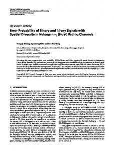
Figure 1: Example of connectivity graph G (left) and associated contention graph W (right). There are six maximal independent sets in W: {(1, 3), (5, 4)}, {(4, 5), (3, 1)}, {(2, 3), (5, 4)}, {(4, 5), (3, 2)}, {(3, 4)}, {(4, 3)} all constraints considered in the primary interference model (also called node-exclusive interference model)—see e.g., [10, 34, 54]—while they are included in the secondary interference model (2-hop interference model) [15, 54]. These interference constraints can be used to create what is oftentimes referred to as contention graph or conflict graph of G; see e.g., [10]. The contention graph W is an undirected graph whose vertices are the directed links of the wireless network, and an edge connects two vertices of W if the corresponding directed links of G cannot be activated simultaneously. The contention graph W can be easily built in a systematic way using the connectivity graph G and the four orthogonality requirements (a)–(d). Fig. 1 illustrates an example of G and W. Once W is known, one can rely on graph-theoretic tools to find the feasible scheduling policies. Specifically, an independent set is a set of vertices in a graph no two of which are adjacent; i.e, it is a set of vertices such that for every two vertices, there is no edge connecting the two. Moreover, a maximal independent set is an independent set that is not a subset of any other independent set; i.e., it is an independent set such that adding any other node to the set forces the set to contain an edge. Based on these definitions, it is clear that two physical links can be simultaneously activated only if they belong to the same independent set of W. Therefore, finding feasible scheduling policies amounts to finding maximal independent sets of W. To rigorously formulate the orthogonality constraints, let s be a maximal independent set of the contention graph W, and S be the collection of all maximal independent sets of W. Since links are allowed to share orthogonally the access to the channel, wsk (h) in [0, 1] will denote the nonnegative fraction of time the links in set s are scheduled per realization h.2 Clearly, the following relationship holds: X wsk (h) ≤ 1, ∀h, k. (2) s∈S 2 Orthogonal

sharing can also be implemented using e.g., orthogonal codes.

7 This way, if wsk (h) = 1, the links in s can transmit during the entire duration of realization h, while links that do not belong to s have to remain silent. On the other hand, if wsk (h) = 0.7 and wsk0 (h) = 0.3, links in s can transmit during the 70% of the duration of realization h, and links in s0 can transmit during the remaining 30%. Time sharing is not necessarily difficult to implement in practice. For example, in existing OFDMA systems, typical bounds on the channel coherence and symbol intervals are 5–100 ms and 5–500 µs, respectively. This means that during a coherence interval several hundreds of symbols are transmitted; hence, those symbols can be assigned to different links. Even so, the ensuing analysis will show that in most situations time sharing is not needed because the optimal scheduling will assign the channel to a single independent set. To account for the fact that a link can belong to different maximal independent sets, let S(i, j) denote the collection of maximal independent sets that contain link (i, j), i.e., k S(i, j) := {s ∈ S : (i, j) ∈ s}, and let wi,j (h) in [0, 1] denote the nonnegative fraction of time the directed link (i, j) is scheduled during the current channel realization. Then it must hold that X k wi,j (h) ≤ wsk (h), ∀h, k, i, j ∈ N (i). (3) s∈S(i,j)

Clearly, optimal allocation requires active links to satisfy (3) with equality. Note also that (2) and (3) need to hold for each and every channel realization. Differently, (1) involves averages over the channel distribution, and therefore it does not depend on a specific h. In the following, constraints that need to hold for all h will be referred to as instantaneous constraints, while constraints that do not depend on the specific realization of h will be referred to as average constraints.

2.3

Physical Layer Operation

The resources adapted at the physical layer are power and rate per link, per channel, and per CSI realization. Specifically, pki,j (h) denotes the instantaneous nominal power transmitted over channel k from node i to node j during the channel realization h. Nominal here means that pki,j (h) is the power that would be transmitted if channel k were allocated to link (i, j) during the entire duration of h. For the general case, where k wi,j (h) ≤ 1, the power effectively transmitted over channel k from node i to node j k during channel realization h is wi,j (h)pki,j (h). Furthermore, two power constraints are considered. On the one hand, the instantaneous power pki,j (h) is bounded by a maximum pre-specified level pˇki,j (spectral mask). On the other hand, the average transmitted power P P k (h)pki,j (h)] cannot exceed a maximum average power budget pˇi . p¯i := E[ k j∈N (i) wi,j Under BER or capacity constraints, rate and power variables are coupled. This ratek power coupling is represented by the function Ci,j (h, pki,j (h)). Similar to the power case, k k k k Ci,j (h, pi,j (h)) represents the nominal transmitted rate, while Ci,j (h, pki,j (h))wi,j (h) is the effective rate transmitted over channel k from node i to node j for the duration of channel k realization h. It is assumed throughout that the rate-power function Ci,j (h, pki,j (h)) is k increasing and strictly concave in pi,j (h). This holds generally for orthogonal access but, for example, not when multiuser interference is present (see Section 7 for details). For k instance, if sufficiently strong error control coding is employed, Ci,j (h, pki,j (h)) is given by Shannon’s capacity formula log(1 + hki,j pki,j (h)/σjk ) [20], which is certainly increasing

8 and strictly concave. Additional examples of concave rate-power functions can be found in [37].

3

Problem Formulation

This section formulates the optimal resource allocation problem. Resource allocation algorithms will be designed so that lower average power consumption and higher exogenous average arrival rates are promoted. To this end, the rate utility functions Uif (·) are selected to be increasing (so that higher rates are promoted) and strictly concave (so that fairness among users and flows is enforced). Similarly, the power cost functions Ji (·) are chosen to be increasing and strictly convex. Note that different utilities may be chosen for different flows f . For example, utility functions that are almost linear are appropriate for best-effort traffic because user satisfaction increases as rate increases. On the other hand, applications such as video streaming with buffering may require the average rate to exceed a minimum prescribed value, and do not experience any significant improvement once that value has been achieved. For this kind of services, concave utility functions can be adopted to yield very high reward for rate increments when the minimum rate has not been achieved, but almost zero reward for rate increments above the minimum rate. Note however that the present formulation does not accommodate real-time traffic with hard delay constraints. Design trade-offs between power cost and rate utility can be accounted for by proper weighting of functions Uif (·) and Ji (·). Taking into account the previous considerations, the optimal channel-adaptive crosslayer resource allocation is obtained as the solution of the following constrained optimization problem: ³ ´ X X P= min − Uif a ¯fi + Ji (¯ pi ) (4a) f a ¯fi ,p¯i ,ri,j (h),

k (h),w k (h),pk (h) wi,j s i,j

subj. to

i

i,f ∈F (i)

X

a ¯fi + X

X

f E[rj,i (h)] ≤

j∈N (i) f ri,j (h) ≤

X

f E[ri,j (h)],

∀i, f ∈ F(i)

(4b)

j∈N (i) k k wi,j (h)Ci,j (h, pki,j (h)),

∀h, i, j ∈ N (i) (4c)

k

f ∈F (i)

  X X k E wi,j (h)pki,j (h) ≤ p¯i ,

∀i

(4d)

k j∈N (i) k wi,j (h) ≤

X

X

wsk (h),

∀h, k, i, j ∈ N (i)

(4e)

s∈S(i,j)

wsk (h) ≤ 1, ∀h, k

s∈S f ri,j (h) ≥ 0, k wi,j (h) ≥ 0, a ¯fi ≥ 0, 0 ≤ pki,j (h) ≤

(4f)

∀h, i, j ∈ N (i), f ∈ F(i)

(4g)

wsk (h)

(4h)

≥ 0,

∀h, k, i, j ∈ N (i), s ∈ S

∀i, f ∈ F(i) pˇki,j , ∀h, k, i, j ∈ N (i);

(4i) 0 ≤ p¯i ≤ pˇi , ∀i.

(4j)

9 The cross-layer nature of the resource allocation problem is apparent because variables of different layers are jointly optimized. The channel-adaptive attribute is also apparent f k since the optimization variables ri,j (h), wi,j (h), wsk (h), and pki,j (h) are all functions of h. The objective in (4a) is constrained to several conditions. Constraints (4g)–(4j) effect lower and upper bounds on different variables, and are known as box constraints, which are easy to tackle. The remaining constraints enforce relationships among variables described in Section 2. Constraint (4b) corresponds to (1) and guarantees the flow conservation. Constraints (4e) and (4f) encapsulate the scheduling decisions at the link layer. Different from (4b) which needs only to hold on average, constraints (4e) and (4f) need to hold for every channel realization h. The interaction among layers is manifested in (4c), which ensures that the number of packets routed during channel realization h never exceeds the instantaneous capacity of the wireless channel. Finally, (4d) represents the average power constraint introduced in Section 2.3. In fact, it can be easily shown that problem with the same solution as (4) could be formulated by replacing p¯i with P aP k E[ k j∈N (i) wi,j (h)pki,j (h)] and eliminating (4d). The reason behind keeping p¯i as a variable in (4d) is that it will be helpful for decoupling the optimality conditions of (4). Problem (4) is nearly convex. In fact, the only source of non-convexity are the monok k k mials wi,j (h)pki,j (h) and wi,j (h)Ci,j (h, pki,j (h)). This source of non-convexity can be elimk inated by introducing the auxiliary variables uki,j (h) := wi,j (h)pki,j (h). It can be shown k that if pki,j (h) in (4) is replaced by uki,j (h)/wi,j (h), the problem becomes convex, and the reformulated problem yields the same Lagrangian as well as the same optimality conditions as those of (4); see e.g., [3, 37, 62]. Since both problems yield the same optimality conditions, the original formulation in (4) will be retained for brevity, without explicitly introducing the auxiliary variables uki,j (h).

4

Optimal Resource Allocation

In this section, the optimal solution of (4) is characterized as a function of the optimal multipliers associated with the constraints in (4), and the instantaneous CSI h. This is accomplished using duality theory in order to find necessary and sufficient conditions for optimality (Section 4.1). The optimal resource allocation schemes at the physical, link, and network layers are developed based on these conditions (Section 4.2). Finally, an alternative solution for asymptotically optimal scheduling and routing schemes is presented and shown to offer distinct advantages relative to the optimal ones (Section 4.3).

4.1

Lagrangian and Optimality Conditions

Using the Lagrangian dual approach, necessary and sufficient conditions that the optimal solution of (4) needs to satisfy are identified in this section. Let ρfi and πi denote Lagrange multipliers associated with the average constraints in (4b) and (4d), respectively. R,f W,k Similarly, let νi,j (h), ϑki,j (h), ξ k (h), ηi,j (h), ηi,j (h), and ηsW,k (h) denote the Lagrange multipliers associated with instantaneous constraints (4c) and (4e)–(4h), respectively.3 Multipliers associated with (4i) and (4j) are not introduced because they are not needed in the subsequent analysis. 3 The

dependence of the multipliers associated with instantaneous constraints on h is written explicitly throughout.

10 Furthermore, let y be a vector containing all the average primal variables, x(h) be a vector containing all the instantaneous primal variables, λ a vector containing all the Lagrange multipliers (dual variables) associated with average constraints, and χ(h) a vector containing all the dual variables associated with instantaneous constraints. The full Lagrangian of (4) is  L(y, x(h), λ, χ(h)) := −

X

Uif (¯ afi )+

i,f ∈F (i)

X

 X

ρfi a ¯fi +

i,f ∈F (i)

f E[rj,i (h)] −

j∈N (i)

X

f E[ri,j (h)]

j∈N (i)

    X X X X k + Ji (¯ pi ) + πi E  wi,j (h)pki,j (h) − p¯i  i

i

X

+

i,j∈N (i)

+

X

k j∈N (i)

 νi,j (h)  

X

X k

X

k (h) − ϑki,j (h) wi,j

X

−

f ∈F (i)

 k k wi,j (h)Ci,j (h, pki,j (h))



wsk (h) +

X

R,f f ηi,j (h)ri,j (h)

i,j∈N (i),f ∈F (i)

X

−

à ξ k (h)

W,k k ηi,j (h) (h)wi,j

X

! wsk (h) − 1

s∈S

k

s∈S(i,j)

k,i,j∈N (i)

−

f ri,j (h)

−

X

ηsW,k (h)wsk (h).

(5)

k,s∈S

k,i,j∈N (i)

Let y∗ , x∗ (h), λ∗ , and χ∗ (h) denote the optimal solution and the associated Lagrange multipliers of (4). Due to the convexity of (4), the Karush-Kuhn-Tucker (KKT) conditions yield the following conditions for optimality [8, Sec. 5.5] (g˙ denotes the derivative of g, and fh (h) the probability density function of random vector h): J˙i (¯ p∗i ) − πi∗ =0

(6a)

−U˙ if (¯ afi ∗ ) + ρfi ∗ k πi wi,j (h)fh (h)dh

=0

(6b)

=0

(6c)

R,f ∗ ηi,j (h)

=0

(6d)

∗ k ∗ k∗ k∗ −νi,j (h)Ci,j (h, pk∗ =0 i,j (h)) + πi pi,j (h)fh (h)dh + ϑi,j (h) − X k∗ k∗ W,k∗ ϑi,j (h) + ξ (h) − ηs (h) =0 −

(6e)

∗ k k −νi,j (h)wi,j (h)C˙ i,j (h, pk∗ i,j (h))

³

ρfj ∗

−

ρfi ∗

´

+

∗ fh (h)dh + νi,j (h) −

W,k∗ ηi,j (h)

(6f)

(i,j)∈s

Conditions (6) must be supplemented with the complementary slackness conditions [8, Chapter 5] and the box constraints in (4i) and (4j). The complementary slackness conditions dictate that if at the optimal point a constraint is satisfied with strict inequality, then the corresponding optimal Lagrange multiplier is zero.

4.2

Characterizing the Optimal Solution

Conditions in Section 4.1 are used to characterize the optimal policies in the present section. To this end, define ρ∗i,j := maxf {ρfi ∗ − ρfj ∗ }, which will play an instrumental role in describing the optimal policies. (The convention ρfi ∗ = 0 whenever i = d(f )

11 k −1 is adopted.) Let also J˙i−1 (·), U˙ if −1 (·) and C˙ i,j (h, ·) denote, respectively, the inverse f k functions of the derivatives of Ji (·), Ui (·), and Ci,j (h, ·). The optimal allocation of average power, average arrival rate, and instantaneous power is described by the following two propositions.4 (Hereafter, [.]ba with a, b real denotes projection onto [a, b], and [.]∞ 0 denotes componentwise projection onto the nonnegative reals.)

Proposition 1 The optimal average power allocation and average arrival rate allocation are, respectively, h ipˇi p¯∗i = J˙i−1 (πi∗ ) (7) 0 h i∞ a ¯fi ∗ = U˙ if −1 (ρfi ∗ ) . (8) 0

The result in (7) follows after solving (6a) with respect to p¯∗i and projecting such solution onto the feasible set [0, pˇi ] defined by the average constraints in (4j). Similarly, (8) follows after solving (6b) with respect to a ¯fi ∗ , and projecting the result onto the feasible set [0, ∞). Note that (8) dictates the flow control implemented at the transport layer. To gain intuition, (8) can be rewritten as U˙ if (¯ afi ∗ ) = ρfi ∗ . The latter reveals that the optimal f∗ flow control policy consists of increasing a ¯i until the marginal utility reaches the cost of injecting more exogenous traffic (measured by ρfi ∗ ) into the network. To ensure stability in practice, one can conservatively select the long-term average rate of each node’s exogenous traffic to stay slightly smaller than a ¯fi ∗ . Proposition 2 The optimal instantaneous power allocation is given by Ã

" pk∗ i,j (h) Interestingly, when

k (h, x) Ci,j

=

k −1 C˙ i,j

= log(1 +

π∗ h, ∗i ρi,j

hki,j x),

!#pˇki,j .

(9)

0

(9) reduces to the well-known waterfilling

pˇk 1/hki,j ]0i,j

∗ k∗ formula pk∗ [20]. For the waterfilling case, higher values i,j (h) = [ρi,j /πi − of πi∗ entail lower power and rate loadings (average power is a limiting factor), while higher values of ρ∗i,j entail higher power and rate loadings (satisfaction of average flow conservation constraint is critical, thus high rates are required). In fact, it is easy to see k that the previous observations hold for any Ci,j (h, ·) increasing and concave. The inverse of the derivative of the rate-power function naturally arises in different power control and resource allocation problems; see, e.g., [6, 29, 37]. While the optimal values p¯∗i , a ¯fi ∗ , and pk∗ ij (h) can be found in closed form, obtaining f∗ k∗ the optimal expressions for ri,j (h), wi,j (h), and wsk∗ (h) is more intricate. The reason for this is that the Lagrangian in (5) is linear with respect to those variables, and dual Lagrangian methods are known to be challenged by linear constraints. k∗ For this reason, before characterizing the optimal wi,j (h) and wsk∗ (h), some definitions are needed. First, for each link consider the functional k ∗ k∗ ϕW (h, k, i, j) := −ρ∗i,j Ci,j (h, pk∗ i,j (h)) + πi pi,j (h) 4 Proofs

(10)

of propositions are not presented due to space limitations. In some cases, a few lines discussing the main idea of the proof are provided.

12 which represents the instantaneous cost of scheduling channel k to link (i, j); that is, the k∗ cost of selecting wi,j (h) = 1. Secondly, for each maximal independent set consider the aggregate functional (1{X} is the indicator function taking the value 1 if expression X is true, and 0 otherwise) X ¡ ¢ ϕS (h, k, s) := ϕW (h, k, i, j)1{ϕW (h,k,i,j) 0, then s∈SS (h,k) wsk∗ (h) = 1; and P k∗ (iii) wi,j (h) = 1{ϕW (h,k,i,j) 0, then f ∈SF (i,j) ri,j (h) = Ci,j (h).

As before, the optimal solution is greedy, meaning that only flows with minimum negative cost are routed. In fact, flows only are allowed to use routes (hops) that decrease the value of the price ρfi ∗ . It can also be verified that the more negative the flow cost in (15) is, the more negative the link channel indicator in (10) becomes. This means that links that could give rise to a significant reduction of the flow cost are more likely to be scheduled. Furthermore, the more negative the flow cost is, the higher the value of the routing variable becomes if the link is scheduled. This is because the power in (9) is higher, thus the capacity is higher. Finally, it is stressed that the gain of a given link does not affect ∗ how different flows share the link, but only Ci,j (h), which represents the total number of packets actually routed through that link. If the minimum cost is attained by a single flow, we have that f∗ ∗ ri,j (h) = 1{f ∈SF (i,j)} Ci,j (h).

(17)

If several flows attain the minimum cost, the specific value for each of the flows can be found using the results of Section 4.3.

4.3

Tie Resolution: Winner-Takes-Almost-All

The event of having different flows (or maximal independent sets) attaining the minimum cost will be henceforth referred to as a tie. The main difficulty in dealing with a tie is that Proposition 3-(ii) and Proposition 4-(ii) do not specify how resources have to be split among winners. The underlying reason is that although any arbitrary splitting minimizes the Lagrangian in (5), only a subset of those splittings (in many cases a single one) is the actual solution to the original constrained problem. One way to find the optimal primal solution when a tie occurs consists of selecting, among all possible tied schedulings (flows), the one that satisfies the average constraints with equality [37]. Although this approach is optimal, it does not lead to a closed-form solution. Furthermore, it requires knowing the exact Lagrange multiplier values; hence it is very sensitive to small inaccuracies. To bypass such problems, we advocate a smooth suboptimal scheme to resolve ties that: (a) can be implemented for any number of elements in SF (i, j) and SS (h, k); (b) is available in closed form (thus incurs reduced computational burden); and (c) is continuous with respect to the Lagrange multipliers. Equally important, the next section establishes analytically that the proposed scheme is asymptotically optimal (meaning that the loss of optimality can be made arbitrarily small). To distinguish the smooth near-optimal

14 schemes developed next from their optimal counterparts, the notation x ˜∗ will be used ∗ henceforth to denote the near-optimal version of the optimal x . The first step to derive the smooth schemes is to realize that the number of elements in SS (h, k) and SF (i, j) is critical to describe the optimal allocation. Since the condition for being a member of those sets is very restrictive (the cost has to be exactly equal to the minimum cost), we relax the definition of sets SS and SF so that more elements belong to them. Specifically, for the case of instantaneous link scheduling, define the minimum independent set cost ϕ∗S (h, k) := min ϕkS (h, k, s0 ). (18) 0 s

Then, we relax the definition of a tie so that now the (suboptimal) collection of independent sets which tie is [cf. (12)] S˜S (h, k) := {s : ϕS (h, k, s) − ϕ∗S (h, k) < εS ∧ ϕS (h, k, s) < 0}

(19)

where εS is a small positive number. Based on S˜S (h, k), the following suboptimal instantaneous link scheduling is proposed:5 ³ 1−

w ˜sk∗ (h) := 1{s∈S˜S (h,k)} P

ϕS (h,k,s)−ϕ∗ S (h,k) εS

³

s0 ∈S˜S (h,k)

X

k∗ w ˜i,j (h) := 1{ϕW (h,k,i,j) 0, then s∈SS (h,k) w ˜sk∗ (h) = 1; and k∗ (iii) w ˜sk∗ (h) and w ˜i,j (h) are continuous functions of λ∗ .

Note that Proposition 5 is true due to definition (20). Properties (i)–(ii) are similar to those in Proposition 3, while (iii) ensures continuity with respect to λ∗ . The sharing coefficient w ˜sk∗ (h) is continuous with respect to ϕS (h, k, s), and the latter is continuous with respect to λ∗ . Proceeding in a similar manner for the instantaneous routing, consider the minimum flow cost ϕ∗F (i, j) := min ϕF (i, j, f 0 ). (22) 0 f

5 From an optimization perspective, (20) is a smooth version of the optimal discontinuous scheduling; see e.g., [69] and [45]. Alternative smooth schedulings, for example based on sigmoidal functions, are also possible.

15 Note that the latter is very similar to the definition of ρ∗i,j given in Section 4.2; specifically, it holds that ρ∗i,j = −ϕ∗F (i, j). Moreover, the set of suboptimal flows is [cf. (16)] S˜F (i, j) := {f : (ϕF (i, j, f ) − ϕ∗F (i, j)) < εF

∧ ϕF (i, j, f ) < 0}

(23)

where εF is a small positive number. Based on S˜F (i, j), we propose the suboptimal instantaneous routing ³ ´2 ϕ (i,j,f )−ϕ∗ F (i,j) 1− F εF f∗ ∗ (h)1{f ∈S˜F (i,j)} P (24) r˜i,j (h) := C˜i,j ³ ´2 ϕF (i,j,f )−ϕ∗ F (i,j) 1 − f ∈S˜F (i,j) εF P k∗ k ∗ (h, pk∗ where C˜i,j (h) := k w ˜i,j (h)Ci,j i,j (h)). The proposed instantaneous routing satisfies the properties described in the next proposition. f∗ Proposition 6 The smooth suboptimal instantaneous routing r˜i,j (h) satisfies: k∗ ˜ (i) If f ∈ / SF (i, j), then r˜i,j (h) = 0; P f∗ ∗ (ii) If |S˜F (i, j)| > 0, then f ∈S˜F (i,j) r˜i,j (h) = C˜i,j (h); and f∗ (iii) r˜i,j (h) is a continuous function of λ∗ .

As before, Proposition 6 is due to (24), and properties (i) and (ii) are similar to those in Proposition 4.

4.4

Layered Resource Allocation

Although the formulation in (4) allows for arbitrary dependence among variables of different layers, it turns out that the optimal schemes presented so far exhibit a layered structure. Indeed, the power and rate loadings at the physical layer depend only on the channel gain and the Lagrange multipliers [cf. (9)]. Once the physical layer is fixed, the links to be activated can be found via (20) and (21); hence, link scheduling does depend on variables of other layers, but in a simple way. With the optimal link and the physical ∗ allocation available, Ci,j (h) can be readily obtained. Then, the network layer can find which flow(s) to route using (24), which requires only knowledge of the Lagrange multipliers. In other words, the way flows share a specific link does not depend on the lower ∗ layers; only the total (aggregate) number of packets is given by Ci,j (h). Finally, the flow f∗ control implemented at the transport layer is based on a ¯i , which according to (8), only depends on the Lagrange multipliers. The intuition behind this solution is that the Lagrange multipliers act as layer interfaces encapsulating all the cross-layer information which is relevant from a resource allocation point of view. These findings are consistent with those in [12] (non-fading case), and in [52] (fading case).

5 5.1

Ergodic Resource Allocation Finding the Optimal Lagrange Multipliers

To implement the optimal resource allocation schemes of the previous section, the optimal multiplier vector λ∗ must be known. However, λ∗ cannot be obtained analytically from

16 the optimality conditions in Section 4.1, and numerical search is needed. This is possible using dual methods. Toward this objective, consider first the partial Lagrangian of (4) where only the contribution of the average constraints is included   X f ³ f´ X f X X f f L(y, x(h), λ) := − Ui a ¯i + ρi  a ¯fi + E[rj,i (h)] − E[ri,j (h)] i,f ∈F (i)

i,f ∈F (i)

j∈N (i)

j∈N (i)

    X X X X k (h)pki,j (h) − p¯i  . + Ji (¯ pi ) + πi  E  wi,j i

i

(25)

k j∈N (i)

Recall that all the instantaneous constraints (link scheduling and instantaneous routing), as well as nonnegativity constraints were already satisfied by the solution of the previous section. Thus, the focus here is to find the Lagrange multipliers associated with average constraints, namely, ρfi and πi for all i, f . With A denoting the feasible set for the primal variables, A := {y, x(h) : (4c), (4e), (4f), (4g), (4h), and (4j) are satisfied}, the dual function is defined as D(λ) :=

inf

(y,x(h))∈A

L(y, x(h), λ) = L(y∗ (λ), x∗ (h, λ), λ),

(26)

which is always concave with respect to λ [4, Sec. 6.2]. Note that y∗ (λ) and x∗ (h, λ) in (26) can be obtained by substituting λ∗ = λ into the expressions of the optimal primal solutions presented in Section 4.2. Based on (26), the dual problem of (4) is D := max D(λ). λ≥0

(27)

Since problem (4) is convex, as long as it is strictly feasible, the duality gap between the primal and dual problems (4) and (27) is zero, i.e., P = D [8, Sec. 5.2]. As a result, the value of λ optimizing (27) can be used to find the optimal primal solution. A standard approach to obtain λ∗ is through a gradient iteration. However, this is impossible here because the linear constraints in (4) render D(λ) non-differentiable with respect to some of the entries of λ. In this case, one can resort to subgradient iterations. For the dual function (26) at a given point λ, it is known that the constraint violation evaluated at the primal solution x∗ (h, λ) and y∗ (λ) is a subgradient [4, Sec. 8.1]. For decreasing and non-absolutely summable stepsizes, subgradient iterations are known to converge in the dual domain [4, Sec. 8.2]. However, for a finite number of iterations finding a (near-)feasible primal solution is not guaranteed. The problem is that f∗ k∗ ri,j (h, λ) and wi,j (h, λ) are typically discontinuous at λ∗ ; therefore, small hovering in the dual domain around λ∗ can give rise to significant differences in the primal domain; see also Section 7.2 for more details about convergence of subgradient iterations. Fortunately, this is not a problem for the suboptimal scheduling and routing of Section 4.3. f∗ k∗ The reason is that when viewed as a function of λ, r˜i,j (h, λ), w ˜sk∗ (h, λ), and w ˜i,j (h, λ) are Lipschitz continuous. (Recall that while for the optimal scheduling the transition from a tie to a single-winner is abrupt, for the suboptimal scheduling the transition is smooth avoiding any discontinuity.) Lipschitz continuity guarantees that proximity in the dual domain implies proximity in the primal domain. In the context of optimization algorithms, smoothing techniques have been successfully used as a mean to effect continuity or differentiability; see e.g., [69] and [45].

17 Before presenting the results for the smooth case, define the smooth version of the dual function as ˜ ˜ ∗ (h, λ), λ) D(λ) := L(y∗ (λ), x

(28)

˜ ∗ (h, λ) are obtained by substituting λ∗ = λ into the expressions of where y∗ (λ) and x the optimal (smooth when needed) primal solutions presented in Sections 4.2 and 4.3. ˜ Similarly, the smooth version of the subgradient is defined as the vector ∂ D(λ) with entries X X f∗ f∗ ˜ f (λ) := a E[˜ ri,j (h, λ)], ∀i, f ∈ F(i) (29) E[˜ rj,i (h, λ)] − ∂D ¯fi ∗ (λ) + ρ i

˜ π (λ) := ∂D i

j∈N (i)

j∈N (i)

  X X k∗  ¯∗i (λ), E w ˜i,j (h, λ)pk∗ i,j (h, λ) − p

∀i.

(30)

k j∈N (i)

Based on these definitions, the following convergence and optimality result follows. Proposition 7 If µ > 0 denotes a small constant stepsize, then for any λ(0) there exists µ so that: (i) the iteration h i∞ ˜ (`−1) ) (31) λ(`) = λ(`−1) + µ∂ D(λ 0

˜ ∗ , i.e., λ(`) → λ ˜ ∗ ; and converges to some point λ ˜ ∗ ) < D(λ∗ ) + f (εS , εF ), where f (·, ·) is a ˜ λ (ii) at the convergence point: D(λ∗ ) ≤ D( positive increasing function satisfying f (εS , εF ) → 0 as (εS , εF ) → (0, 0). Proposition 7 has various implications. As far as convergence is concerned, it provides ˜ ∗ . From a feasibility perspective, it guarantees that a systematic algorithm to compute λ ∗ ∗ ˜ ˜ (h, λ) is implemented at λ , the average flow conservation and power constraints if x ˜ are satisfied with equality (recall that ∂ D(λ) = 0 only if this holds). Finally, from an optimality perspective, it guarantees that the overall price paid for implementing the smooth instead of the optimal policy is asymptotically small.6 . The last assertion is true because the bounds on the dual values given in Proposition 7-(ii), directly translate to bounds on the objective in (4a). A rigorous proof of this proposition for a problem related to the one investigated in this chapter can be found in [37].

5.2

Operational Mode: Offline and Online Phases

The proposed cross-layer channel-adaptive schemes operate in two phases: (a) an offline phase, which takes place before communication starts during the initialization phase; and (b) an online phase, which is executed during the communication process, every time the instantaneous CSI h is updated. ˜ ∗ . As preThe main objective of the offline phase is to find the Lagrange multipliers λ ∗ ˜ is found through (31), which basically describes dual subgradient sented in Section 5.1, λ 6 In practice, the gap with respect to D(λ∗ ) is almost zero even for finite (small) values of ε and ε . S F This is true because the smooth schemes are slightly suboptimal only when ties occur, which are rare events.

18 iterations. It is known that such methods may have slow convergence in practice. Hence, hundreds of iterations may be needed in order to find Lagrange multipliers reasonably close to the optimal ones. Of course, the specific number of iterations depends on factors such as the initialization point, the stepsize, and the required accuracy. Moreover, the computational burden for each iteration can be high, especially for large-scale networks. The reason is that the subgradients in (31) involve expectations over the channel distribution [cf. (29) and (30)]. In practice, these expectations are replaced by Monte Carlo estimates. The samples needed for this may be obtained (a) by drawing independent realizations from the distribution of h, if it is known; or (b) by using actual channel measurements, if such are available. Method (b) works even if the measurements are correlated—which may happen in the present context when the fading process is correlated across time. In any case, the higher the size of the network is, the bigger the number of channel realizations needed to obtain a reliable estimate of the actual subgradients becomes. It is also worth mentioning that for each channel realization, the independent set of links that wins access to the channel needs to be found. Enumerating all maximal independent sets has in general exponential complexity; see e.g., [54]. Different from other scheduling schemes, as in e.g., [10, 34], such a computation here needs to be executed only once, before the offline phase starts. All maximal independent sets are identified upon the initialization, and for each channel realization generated, the independent set achieving the highest link quality indicator can be easily found. It should finally be stressed that although the offline phase incurs high computational burden, it only needs to be re-run every time the channel statistics or the system set-up changes. In contrast, the online phase needs to be executed every time the CSI changes, which depends on the channel coherence interval. Then, based on the current value of the CSI ˜ ∗ obtained from the offline phase, the resources at the different layers h, and the value of λ are adapted according to (9)–(24). Note that in the online phase, there is no need for re-computing S, since it is already available from the offline phase. Although the optimal allocation at the physical and network layers only requires local CSI, obtaining the optimal link activations requires knowledge of the full h vector. Specifically, to find the optimal scheduling, the maximal independent set giving rise to the lowest cost needs to be found. To this end, nodes need to share either the channel gains of their local links, or, the value of their link cost indicators. Exchange of this information can be implemented using different options. In a decentralized approach, control channels may be available, over which nodes exchange their local information—see [3] for a protocol that implements this task. Under a hierarchical approach, the network can contain scheduler-node(s)—regular or dedicated—that gather the information, find the optimal link allocation, and broadcast it to the transmitting nodes.

5.3

Numerical Example

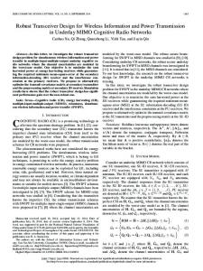
To illustrate how the developed schemes perform, numerical tests were simulated for the very simple case of the network in Fig. 2(a) involving I = 3 nodes, all of them connected. Moreover, F = 3 different flows—one for each possible destination—and K = 4 parallel channels are considered. The channel SNRs are exponentially distributed, their average power gain is 5 dB, and are assumed to be reciprocal (i.e., hki,j = hkj,i ). The utilities to be maximized are Uif (x) = log(1+x), if (i, f ) = (1, 3) or (i, f ) = (3, 2); Uif (x) = log(1/10+x), if (i, f ) = (2, 1); and zero for all other node-flow combinations. The power cost functions

19

(a)

(b)

Figure 2: Network with 3 nodes, all connected with each other. For the first test case, all channels have the same SNR (left). For the second test case, the channel between nodes 2 and 3 is very weak (right). are Ji (x) = x2 /10 forall i. Moreover a maximum average transmit power of pˇi = 5 per node is considered. The performance of the network during the online phase when the optimal multipliers ¯23 = 3.0; ¯12 = 2.6, a are used is the following: p¯1 = 1.5, p¯2 = 1.3, p¯3 = 1.5; a ¯31 = 3.0, a 2 1 3 and r¯1,3 = 3.0, r¯2,1 = 2.6, r¯3,2 = 3.0; and zero for all other variables. Note first that the network conditions are similar for nodes 1 and 3. This is not true for node 2, because it routes packets from flow 1, which according to the utilities considered, yield lower utility. Taking into account these facts, we observe that the numerical results follow the expected behavior since power and rate performance are similar for nodes 1 and 3; and the optimal exogenous rate injected at node 2 is smaller than that at nodes 1 and 3. To further validate the developed schemes, we slightly modify the set-up and reduce the average channel gain between nodes 3 and 2 by 10 dB. The modified configuration yields 3 = 2.6, ¯23 = 1.5; and r¯1,3 ¯12 = 2.3, a the following: p¯1 = 1.8, p¯2 = 1.3, p¯3 = 1.2; a ¯31 = 2.6, a 2 2 2 1 r¯2,1 = 2.3, r¯3,2 = 0.3, r¯3,1 = 1.2, r¯1,2 = 1.2; and zero for all other variables. Since the channel between nodes 3 and 2 is now very poor, most of the packets from 3 destined for 2 are routed through 1. Indeed, this is confirmed by the numerical results. Moreover, we also observe that the power consumed by node 1 increases, the exogenous rate injected at node 3 decreases, and the overall network performance decreases. Clearly, all these changes are caused by the SNR loss between nodes 3 and 2.

6

Stochastic Resource Allocation

The resource allocation algorithms developed in the previous sections are functions of two variables: the current CSI h, and the optimal (smooth) Lagrange multipliers. As men˜ ∗ offline requires knowledge of the channel distribution, and incurs tioned earlier, finding λ considerable computational burden. To bypass these challenges, resources can be allocated using stochastic approximation algorithms. These algorithms learn the unavailable information on-the-fly, exhibit tracking capabilities, and incur moderate computational complexity. Roughly speaking, they could be understood as “intelligent” least mean-square (LMS) type schemes. From an operational perspective, they operate as fully on-line solutions because they do not require offline calculations and consume limited computational resources. Different alternatives can be considered to develop such stochastic schemes.

20 The approach here is to implement the cross-layer resource allocation not based on the optimal Lagrange multipliers, but on a stochastic estimate of them that varies with time ˜ ∗ is replaced by λ[n]. ˜ n; i.e., λ It is important to clarify that n indexes blocks whose duration is the channel coherence interval. In other words, the resource allocation and the Lagrange multiplier estimates are updated every time the CSI h = h[n] is updated. Recall that the fading process {h[n]}∞ n=1 is assumed to be stationary and ergodic. On top of coping with channel nonstationarities and reducing the computational burden, the stochastic algorithms facilitate distributed implementation, and link Lagrange multipliers with queue lengths analytically. This link is exploited in upcoming sections to: (a) characterize the average queueing delay of the stochastic schemes and, consequently, enable a way to incorporate explicitly the delay into the design; and (b) create links with existing algorithms that allocate resources based on the state of the queues.

6.1

Estimating the Lagrange Multipliers

The first step to obtain the stochastic schemes consists of replacing the original ensemble iterations in (29) and (30) with their instantaneous counterparts. Specifically, a Robbins˜ Monro approach is used to obtain λ[n], whereby all ensemble average terms in (29) and (30) are replaced by unbiased instantaneous (one-shot) estimates, as in e.g., [24]. ¡ ¢ ˜ Specifically, with afi ∗ n, λ[n] denoting the instantaneous arrival of flow f at node i during block n [which is a random variable drawn for a distribution with mean a ¯∗m (λ[n])], the following iterations are proposed: X f∗ X f∗ ¡ ¢ ˜ ˜ ˜ ˜ ˜ f (n, λ[n]) := afi ∗ n, λ[n] + [˜ rj,i (h[n], λ[n])] ∂D − [˜ ri,j (h[n], λ[n])] (32) ρ i

j∈N (i)

j∈N (i)

  X X k∗ k∗ ˜ ˜ ˜ ˜ ˜ π (n, λ[n])  ¯∗i (λ[n]) ∂D :=  w ˜i,j (h[n], λ[n])p i,j (h[n], λ[n]) − p i

(33)

k j∈N (i)

where (32) does not apply if i = d(f ). Comparing (32) and (33) with (29) and (30), the expectations over h have indeed been dropped, and the ensemble λ has been replaced ˜ ˜ has been with its stochastic estimate λ[n]. Moreover, the optimal average arrival a ¯fi ∗ (λ) ¡ ¢ f∗ ˜ replaced by its stochastic counterpart ai n, λ[n] . Key to convergence analysis is that ˜ ˜ λ (n, λ[n])} sequence {∂ D is bounded, which is true as far as both the instantaneous rates i at the physical level and the exogenous instantaneous arrival rates at the network level ˜ ˜ ˜ λ (n, λ[n])] ˜ λ (λ[n]), are bounded. In addition, it holds by construction that E[∂ D = ∂D i i where the expectation is conditioned to the history of the network; i.e., {h[r]}nr=0 and n ˜ {λ[r]} r=0 . Based on the previous definitions, the original iterations over λ in (31) are replaced by their stochastic counterparts h i∞ ˜ + 1] = λ[n] ˜ + µ∂ D(n, ˜ ˜ λ[n λ[n]) (34) 0

where µ > 0 denotes again a constant stepsize. Equation (34) shows clearly that now ˜ λ[n] depends on the random value of h[n], thus it is stochastic. Once the stochastic multipliers are available, they are substituted into the primal optimal solution presented in Section 4, to yield the stochastic version of the primal

21 solution. Specifically, the stochastic version of the optimal average power, average arrival rate, and instantaneous power per time slot n are, respectively, h ipˇi ˜ p¯∗i (λ[n]) := J˙i−1 (˜ πi [n]) , 0

h ˜ a ¯fi ∗ (λ[n]) := U˙ if

i∞ (˜ ρfi [n])

−1

h i ˜ ˙ k −1 (h[n], π pk∗ ˜i [n]/˜ ρi,j [n]) i,j (h[n], λ[n]) := Ci,j

0

pˇk i,j 0

(35) (36)

Similarly, the stochastic versions of the suboptimal instantaneous scheduling and routing are given by Ã

!2 ˜ ˜ ϕS (h[n], λ[n], k, s) − ϕ∗S (h[n], λ[n], k) := 1{s∈S˜S (h[n],λ[n],k)} 1− ˜ εS , Ã !2 X ˜ ˜ k) ϕS (h[n], λ[n], k, s0 ) − ϕ∗S (h[n], λ[n], 1− (37) εS ˜ s0 ∈S˜S (h[n],λ[n],k) X k∗ ˜ ˜ w ˜i,j (h[n], λ[n]) := 1{ϕW (h[n],λ[n],k,i,j) 0, there exist bT > 0 and µT > 0 so that max

1≤n≤T /µ

˜ kλ(n) − λ[n]k ≤ cT (µ)bT ,

0 ≤ µ ≤ µT

with probability 1

(41)

7 The locking results provided in the proposition can be shown based on the averaging approach ˜ with respect to λ ˜ can be ˜ in [56, Chapter 9]. The main idea is that the Lipschitz continuity of ∂ D(n, λ) used to prove that the most challenging conditions required in [56, Theorem 9.1] hold. A similar approach can be used to show the convergence in probability result in (42) when n → ∞ [56, Theorem 9.5].

22 where cT (µ) → 0 as µ → 0. (ii) Given A > 0, there exists a random variable W (µ) so that ˜ max Pr{kλ(n) − λ[n]k > A} ≤ Pr{W (µ) > A} n≥1

(42)

where W (µ) → 0 as µ → 0 with probability 1. Proposition 8 states that the dual iterates do not strictly converge to the optimal value but may hover around it. Since the resource allocation is a function of the stochastic multipliers, the stochastic version of the instantaneous primal variables (36)–(40) exhibit the same convergence behavior. This means that the stochastic instantaneous primal variables may hover around their optimal (non-stochastic) counterparts; e.g., k∗ ˜∗ ˜ pk∗ i,j (h[n], λ ) 6= pi,j (h[n], λ[n]) even when n → ∞. The convergence of the primal iterates is characterized next, in terms of their sample averages.8 Proposition 9 The sample average of the stochastic resource allocation: (i) is feasible and (ii) entails a small loss of performance relative to the average non-stochastic solution of the problem in (4). Specifically, as n → ∞, it holds with probability 1 that   n n i X 1 X  X h f∗ f∗ ˜ ˜ ˜  ≥ 1 (i) r˜j,i (h[r], λ[r]) a ¯f ∗ (λ[r]) − r˜i,j (h[r], λ[r]) n r=1 n r=1 i j∈N (i)   n n 1X ∗ ˜ 1 X X k∗ k∗ ˜ ˜  w ˜i,j (h[r], λ[r])p (h[r], λ[r]) ≤ p¯ (λ[r])) i,j n r=1 n r=1 i

(43)

(44)

k,j∈N (i)

(ii) With δP (µ) denoting a small number proportional to the stepsize µ

−

Ã

X

Uif

i,f ∈F (i)

! Ã n ! n X 1 X f∗ ˜ 1X ∗ ˜ ˜ ∗ + δP (µ). Ji a ¯ (λ[r]) + p¯i (λ[r]) ≤ P n r=1 i n r=1 i

(45)

In other words, both stochastic and non-stochastic allocations are asymptotically (δP (µ)) optimal when n → ∞. Of course, differences between the offline/online (non-stochastic) schemes presented in Section 5 and the fully online (stochastic) schemes presented in Section 6 arise also on issues such as speed of convergence to the optimal average values, or, sensitivity to changes in the channel realization, to name a few. Equally relevant, convergence results can also be obtained when the averages in (43)(45) are not defined as sample averages. For example, if they are defined using a finite-size sliding window averaging, or, as an exponentially decaying average, then convergence in distribution to a Gaussian random variable whose mean is the optimal solution of (4) can be shown. A rigorous proof along with characterization of the variance of the Gaussian distribution can be obtained using the results in [24, Chapter 11]. 8 Propositions

9 and 10 can be proved using the results in [7, 24, 49].

23 Remark 1 Although not presented here, stochastic implementations different that those in (32)–(34) can be proposed. These include variations with decreasing stepsizes, and replacement of the ensemble averages with windowed averages or sample averages; see [39, 61] for examples. Needless to say, the convergence claims in each of those cases are different (stronger) than those presented here. As it is shown in the next section, we focus here on the simpler implementation of (32)–(34), because it allows us to establish connections with queuing theory and existing resource allocation algorithms.

6.2

Queue Stability and Average Delay

Communication systems are typically equipped with queues that store packets from higher layers. Packets leave the queues with a rate that depends on the state of the channel and the resource allocation decisions. So far, such queues have been only indirectly accounted for in the problem formulation via (1), where average flow conservation constraints have been imposed as a necessary condition for stability. In what follows, the queue stability and the delay performance of the stochastic resource allocation algorithms will be characterized. Characterizing the queuing delay in adaptive systems operating over fading channels is typically complicated because most of the standard assumptions do not hold. Indeed, departure times are typically correlated, and the distributions for the arrival and departure times are difficult to describe because they depend on the resource allocation algorithm and the underlying channel fading distribution. This is the case for the non-stochastic online algorithm developed in Sections 4 and 5. It will be nevertherless seen soon that the analysis for the stochastic algorithms is tractable. Moreover, the full buffer assumption (cf. Section 2.1) was required for non-stochastic algorithms to be stable, but it is not needed for their stochastic counterparts. Starting with the analysis of queue dynamics, let qif [n] denote the queue size for flow ˜ f at node i at the time slot n. Moreover, recall that afi ∗ (n, λ[n]) stands for the random instantaneous arrival, which is drawn for a distribution with mean a ¯∗m (λ[n]) given by (35). Then, the queue obeys for all f and all i 6= d(f ) the recursion  ∞ X X f∗ f∗ ˜ ˜ ˜  , qif [n + 1] = qif [n] + afi ∗ (n, λ[n]) + [˜ rj,i (h[n], λ[n])] − [˜ ri,j (h[n], λ[n])] j∈N (i)

j∈N (i)

0

(46) In practice, arrivals and departures are magnitudes that vary in a time scale smaller than n. This implies that definitions slightly different from the one in (46) are also possible (e.g., one could alternatively say that packets arriving in time slot n can only be transmitted in time slot n + 1). Such differences are not relevant for the subsequent analysis and, as it will be apparent next, (46) has been chosen for simplicity. At this point it is useful to particularize the stochastic iteration in (34) for the specific case of ρfi [n + 1] (recall that ρfi is the Lagrange multiplier associated with the flow conservation constraint of flow f at node i). According to (32) and (34), such iteration is   ∞ X X f∗ f∗ ˜ ˜ ˜  ρ˜fi [n+1] = ρ˜fi [n] + µ afi ∗ (n, λ[n]) + [˜ rj,i (h[n], λ[n])] − [˜ ri,j (h[n], λ[n])] j∈N (i)

j∈N (i)

0

(47)

24 for all f and i 6= d(f ). Comparing (47) with (46), it is clear that ρfi [n] and qif [n] are related in a way that the stochastic Lagrange multipliers can be interpreted as scaled values of the queue lengths. Specifically, if ρfi [0] = µqif [0], then it follows that qif [n] = ρfi [n]/µ. Had the definition of the queue update in (46) been different, one could always bound the instantaneous difference between qif [n] and ρfi [n] for all n, and argue that after an initial transient period, the approximation qif [n] ≈ ρfi [n]/µ would be accurate. The previous finding is meaningful from different points of view, namely, (a) analyzing stability of the resource allocation algorithms; (b) estimating the queueing delay that packets will experience; and (c) establishing connections with other well-known crosslayer resource allocation algorithms. The ensuing subsections briefly elaborate on those issues. 6.2.1

Queue Stability

To analyze stability of the stochastic resource allocation in (34)–(40), the fact that qif [n] = ρfi [n]/µ implies the following result about the convergence of the sample average of the queue lengths. Pn Proposition 10 If q¯if [n] := n−1 r=1 qif [r] denotes the sample average of the queue size qif [n] and δq is a small number proportional to the maximum update in (34), then |qˆ¯if [n] − ρ˜∗i /µ| < δq as n → ∞

w.p. 1.

(48)

Therefore, it holds that when n grows large, q¯if [n] is finite provided that ρ˜fi ∗ is finite, which is guaranteed if the original problem is feasible. It is worth noting that although Proposition 10 establishes convergence of the sample average of the queue lengths to a finite value, bounds on the instantaneous size of the queues can also be characterized using the Lagrange multipliers bounds given in Proposition 8. 6.2.2

Average Delay

The relationship between queues and Lagrange multipliers can also be used to estimate the average queueing delay that the proposed stochastic resource allocation incurs. To this end, one can invoke Little’s result [23] that asserts that with stable queues, the average delay is given by the average aggregate queue length divided by the average aggregate arrival rate. This implies that the average delay of a flow (say f ) in the entire network is P f q¯ f ¯ d := Pi if ¯i ia

(49)

where in (49), q¯if generically denotes the expected length of the queue that node i keeps f for flow f . Moreover, with r¯j,i denoting the average routing variable, the average delay experienced by packets of flow f while waiting in the queue of node i is d¯fi :=

a ¯fi

+

q¯if P

f ¯j,i j∈N (i) r

.

(50)

25 Using the results in Proposition 10, it readily follows that the average delays for the stochastic resource algorithms presented in this chapter can be approximated as, d¯f

≈

P f∗ ρ˜i 1 P if ∗ ˜ ∗ µ ia ¯i (λ )

(51)

d¯fi

≈

1 ρ˜fi ∗ . f∗ ˜ ∗) + P ˜ ∗ )] µa ¯fi ∗ (λ rj,i (h, λ ∀j∈N (i) E[˜

(52)

In other words, the average delay of the stochastic algorithm can be estimated from the optimal solution of (4) and the stepsize of the proposed iterations. Changing the Stepsize: Upon examining (51) and (52), it is apparent that changes in the stepsize induce changes in the average delay. Specifically,(51) and (52) reveal that the higher the stepsize, the smaller the average queuing delay. The intuition behind this is that high stepsizes will accelerate convergence and thus improve the ability to react against events that otherwise would increase the queuing delay. However, high stepsize values will also lead to more pronounced hovering in the dual domain, and may endanger convergence and stability if they are set beyond a certain level. Besides quantifying the average delay, the expressions in (51) and (52) are also useful to effect delay priorities. Key for this purpose is the fact that the iterations in (31) and ˜ but also if the stepsize (34) converge not only if the stepsize is common to all entries of λ, is different for each entry. This way, flows and nodes with stricter delay constraints can use a larger stepsize. In a nutshell, if one allows the stepsize to be dependent on i and f , then different delay performances can be obtained. Sensitivity Analysis: Another issue of interest is to know how delay varies when any of the variables present in (4) is modified. This is non-trivial because in most cases ρ˜fi ∗ is not available in closed form, and even if it is, its dependence on other parameters is difficult to characterize. Convex optimization tools can be used to decipher properties of ρ˜fi ∗ . Specifically, to rigorously study the effect of modifying variables present in (4) on the average delay of our algorithms, sensitivity analysis has to be used. This analysis is typically complex, although there are a few cases where it can be tractable. For the problem at hand, this is the case for the arrival exogenous rate a ¯fi ∗ . In fact, if a node i accepts exogenous packets of a given flow f , the KKT conditions can be used to show that ρ˜fi ∗ = U˙ if (¯ afi ∗ ). The latter implies that d¯fi ≈ µ−1 U˙ if (¯ afi ∗ )/¯ afi ∗ . Upon differentiating, it f∗ ¨ f (¯ follows that ∂ d¯fi /∂¯ afi ∗ ≈ U afi ∗ − U˙ if (¯ afi ∗ )/(¯ afi ∗ )2 . This implies that ∂ d¯fi /∂¯ afi ∗ < 0, i ai )/¯ because utilities are concave and increasing. As a result, we deduce that problems giving rise to higher a ¯fi ∗ , exhibit lower delay. Space limitation prevents further elaboration on this subject.

6.3

Cross-Layer Design and Dynamic Backpressure

Section 4.4 demonstrated that the developed cross-layer schemes exhibit a layered structure, and also that interaction among layers is mainly encapsulated by the Lagrange multipliers ρfi ∗ and πi∗ . For the schemes in Section 6, one can go one step further in the interpretation of these multipliers. In fact, the results of Subsection 6.2.1 revealed that a scaled version of the queue length provides an unbiased estimate of ρfi ∗ . Changes in the queue lengths (thus changes in ρfi [n]) induce changes in the allocation of resources

26 at all layers. Specifically, node-flow pairs with large queues give rise to: (a) reduced exogenous and high outgoing endogenous rates (transport and network layers), (b) high link quality indicator (link layer), and (c) high power and rate loadings (physical layer). Similarly, changes at the physical layer (e.g., changes in the channel gains) induce changes of resource allocation at physical, link, and network layers. A major implication of the relationship between the stochastic Lagrange multipliers and queue sizes revealed in Subsection 6.2.1 is that the developed schemes are stable. This was not guaranteed at the outset because queue stability was never explicitly imposed in the present formulation. (Recall that the average flow conservation condition imposed via (1) is necessary but not sufficient.) An intuitive explanation for this behavior is that the developed schemes adapt resources at different layers to react against short-term changes in the state of channels and queues. This way, if the instantaneous arrival rates of a given flow happen to be high or the channel gains happen to be low during several block indices, then the adaptive schemes react to increase the transmit-power, select that flow to be routed, and reduce the average exogenous rate. All those decisions clearly contribute to network stabilization. Equally important, the relationship between the stochastic Lagrange multipliers and queue sizes is also useful to draw connections between the schemes presented in this chapter and the celebrated dynamic backpressure algorithm. This algorithm was proposed in [58], and later extended to fading networks with cross-layer adaptation [18]. Instead of using dual optimization theory, the schemes in [18] are derived using a Lyapunov stability approach (actual and virtual queues are inputs of the Lyapunov function) under which the resource allocation objective is to stabilize the network. Comparing the results here with those in [18], it easy to infer that: (a) the optimal routing schemes are the same in both cases; and (b) the optimal resource allocation schemes at the link and physical layers are related, with the main difference being that the role which is played here by the Lagrange multipliers, is played by the virtual queues and tuning parameters in [18].

7

Non-Orthogonal Access

In the present section, the focus shifts to multi-hop wireless networks with non-orthogonal access. The main difference here is that all nodes are allowed to access the available tones simultaneously, treating the interfering transmissions as noise. An advantage of using a non-orthogonal approach is that scheduling becomes implicit in the power allocation. k Therefore, there is no need for introducing the scheduling variables wi,j (h) and wsk (h)— recall that in the orthogonal case it was necessary to find the collection of all maximal independent sets, which has exponential complexity. A disadvantage is that the optimization problem for non-orthogonal access is generally non-convex, and may again incur exponential complexity. Non-convexity emerges because now the instantaneous capacity of each link depends on the SINR of that link, which couples the power allocation decisions. Non-convexity typically brings two undesirable effects: (a) there may not be efficient algorithms to find the optimal solution; and (b) using a dual approach to solve the problem is not optimal, because zero duality gap is not guaranteed. Section 7.1 gives the optimal networking formulation with the SINR-limited physical layer, and corresponds to material of Sections 3 and 4. Then, an ergodic resource allocation algorithm is presented in Section 7.2, which is the counterpart of the one given

27 in Section 5 for the orthogonal case. Stochastic resource allocation algorithms are not presented here; the interested reader is referred to [49]. An alternative online algorithm is presented in [48]. Many of the model parameters and network design variables, such as the exogenous arrival rates a ¯fi , coincide with those for orthogonal access. These are only cursorily mentioned here; see Section 2 for more elaboration. On the other hand, the differences between the two models are stressed throughout this section. The content of this section draws mainly from material reported in [17, 52], and the proofs for all results in the present section can be found in these works.

7.1

Problem Statement and Duality Properties

The cross-layer resource allocation problem for multi-hop networks with non-orthogonal access is formulated in Subsection 7.1.1, while a fundamental property of the optimization problem is stated in Subsection 7.1.2 using Lagrangian duality. 7.1.1

Problem Statement

The formulation developed here considers the long-term average rate of flow f from node f i to node j, r¯i,j , instead of the instantaneous one; see also [18]. Note that this approach is f (h) not essential in the case of non-orthogonal access treated here; a formulation using ri,j would also be possible. The flow conservation constraint corresponding to (1) or (4b) is X f X f a ¯fi ≤ r¯i,j − r¯j,i , ∀i, f ∈ F(i). (53) j∈N (i)

j∈N (i)

The total average rate carried by any link cannot exceed the average capacity of the link, c¯i,j ; this leads to the link capacity constraint X f r¯i,j ≤ c¯i,j , ∀i, j ∈ N (i) (54) f ∈F (i)

which can be viewed as a long-term average version of (4c). Note that there is no quantity in (4) corresponding to c¯i,j . Variables c¯i,j represent the average data rates at the link layer, and they are related to the instantaneous capacities, as described next. Link capacities are dictated by the SINR at the physical layer, whereby different nodes are allowed to use the same frequency to transmit and treat other nodes’ transmissions as noise. This is the case when receiving nodes implement single-user decoding. The instantaneous SINR of link (i, j) over tone k is k γi,j (h, p(h)) :=

σjk +

P

hki,j pki,j (h) (κ,l)∈Ii,j

hkκ,j pkκ,l (h)

(55)

where σjk is the noise variance at node j over tone k, and Ii,j denotes the set of links causing interference to (i, j). This set consists of the links carrying: (a) incoming transmissions for j over k from nodes other than i, (b) outgoing transmissions from j, and (c) transmissions originating from nodes in N (j) intended for nodes other than j. Hence, this set takes the form © ª Ii,j := (κ, l): κ ∈ N (j)\{i}, l ∈ N (κ); (i, l): l ∈ N (i)\{j}; (j, l): l ∈ N (j) . (56)

28 P Based on (56), the term hkj,j l∈N (j) pkj,l in the denominator in (55) represents selfinterference to receiving node j from transmissions originating from j. In order to discourage this self-interference, and thus ensure half-duplex operation of the nodes, hkj,j is set to a high (deterministic) value. Furthermore, interference from “far-away” links, corresponding to (κ, l) with κ ∈ N (j), κ 6= j and l ∈ N (κ), l 6= j, is neglected. Note that all links causing interference to link (i, j) are explicitly accounted for in the orthogonal f transmissions constraints considered in Section 2.2. Moreover, the SINR γij depends on power allocation p(h) as well as on h. Whenever needed, the latter is emphasized by f writing γi,j (h, p(h)). It is important to remark at this point that P-CSI is assumed throughout Section 7. The reason is that the subsequently developed results rely on the fact that the fading is continuous. This is of course true for P-CSI, but not when Q-CSI is available because h is then a discrete random vector. The transmission rate (instantaneous capacity) of link (i, j) over tone k is described k k via a generic function of the SINR over that link and tone, Ci,j (γi,j ), which is increasing and concave in the SINR. The instantaneous capacity depends on power allocation p(h) as well as on h, because the SINR depends on those [cf. (55)]. This function is the k counterpart of Ci,j (h, pki,j (h)) in Section 2.3. Note though that the rate of link (i, j) here depends on the power allocations over all neighboring links—via the SINR—and not only on the power allocation over link (i, j), as was the case with the orthogonal access. A few k k particular examples of Ci,j (γi,j ) are now in order. k k Supposing Gaussian codebooks with sufficiently large blocklengths, Ci,j (γi,j ) takes the form ¡ ¢ k k k Ci,j (γi,j ) = log 1 + γi,j . (57) It is also possible to include a penalty term in (57), called SINR gap, Γ, in order ¡ tokaccount ¢ k k for practical codes and adaptive modulation schemes [20]: Ci,j (γi,j ) = log 1 + γi,j /Γ . Furthermore, a high-SINR approximation of (57) can also be used for cross-layer optimization ¡ k k ¢ k k Ci,j (γi,j ) = ln Ki,j γi,j (58) k where Ki,j is a constant. It should be stressed that (58) is meaningful only when k k γi,j > 1/Ki,j ; otherwise the logarithm is a negative number. A more general model k k which includes (58) as a special case considers a strictly increasing Ci,j (γi,j ) satisfying the condition k k k k k k C¨i,j (γi,j ) · γi,j + C˙ i,j (γi,j ) ≤ 0, ∀ γi,j > 0. (59)

A linear function of the SINR (low-SINR approximation) is another model: k k k k Ci,j (γi,j ) = Ki,j γi,j

(60)

k where Ki,j is a constant. The previously mentioned forms of the capacity function (57)– (60) have been used for cross-layer optimization in [11, 13, 17, 19, 33, 34, 43, 47, 64, 65]. The ergodic capacity c¯i,j of link (i, j) is

" c¯i,j := E

X k

# k k Ci,j (γi,j (h, p(h))) .

(61)

29 As in Section 3, two kinds of power constraints are considered. The first are instantaneous spectral mask constraints, expressed as 0 ≤ pki,j (h) ≤ pˇki,j , as in (4j). Second, the average power consumed by a node in the network [cf. (4d)] is   X X p¯i := E  pki,j (h) (62) j∈N (i) k

is constrained by a power budget pˇi , i.e., 0 ≤ p¯i ≤ pˇi for all i, as in (4j). Average exogenous rates a ¯fi in practical networks lie within application-specific bounds f f f expressed as ai min ≤ a ¯i ≤ ai max . Furthermore, the network designer may wish to impose f upper bounds on link capacities c¯i,j and multicommodity flows r¯i,j , that is 0 ≤ c¯i,j ≤ cˇi,j f and 0 ≤ r¯i,j ≤ rˇi . Note that such upper bounds are not used in the formulation of Section 3 [cf. (4g)], but they could have been included, leading also to appropriate modifications of Propositions 4 and 6. As in Section 4, the notation y is used to denote the collection of f all average variables, namely, a ¯fi , r¯i,j , c¯i,j , and p¯i for all i, j ∈ N (i), f ∈ F(i). Then, the previously mentioned box constraints are summarized by the polyhedral set B:={y, p(h) : 0 ≤ pki,j (h) ≤ pˇki,j , 0 ≤ p¯i ≤ pˇi , f ¯fi ≤ afimax , 0 ≤ c¯i,j ≤ cˇi,j , 0 ≤ r¯i,j ≤ rˇi}. afimin ≤ a

(63)

Increasing and strictly concave utility functions Uif (¯ afi ) for the exogenous arrival rates, and increasing and strictly convex cost functions Ji (¯ pi ) for the average powers will be used. The optimal networking problem is [cf. (4)] X X Uif (¯ afi ) − Ji (¯ pi ) (64a) P = max (y,p(h))∈B

subj. to

i

i,f ∈F (i)

a ¯fi

X

≤

X

X

f r¯j,i ,

"

X k

X X

∀i, f ∈ F(i)

(64b)

∀i, j ∈ N (i)

(64c)

∀i, j ∈ N (i)

(64d)

∀i.

(64e)

j∈N (i)

f r¯i,j ≤ c¯i,j ,

c¯i,j ≤ E E

−

j∈N (i)

f ∈F (i)

"

f r¯i,j

# k k Ci,j (γi,j (h, p(h)))

# pki,j (h) ≤ p¯i .

j∈N (i) k

A comparison between (4) and (64) is due now. The objective (64a) corresponds to (4a). Constraints (64b) and (64e) parallel (4b) and (4d), respectively. Furthermore, there are no constraints corresponding to (4e), (4f), and (4h), as there are no scheduling variables here. The counterparts of constraints (4g)–(4j) are included in B. Moreover, constraints (64c) and (64d) combined correspond to (4c)—note that there is also an additional variable here, namely c¯i,j . Introduction of c¯i,j as optimization variable is not essential, but offers the advantage of providing an interface between the network layer f k k average flows r¯i,j and the instantaneous physical layer capacities Ci,j (γi,j ). In practice, the traffic flowing in the network is stored in queues. The constraints in (64) are necessary conditions for stability [18]. The queueing operations in the network

30 and how the solution of (64) can be used for network control is described in detail in Subsection 7.2.3. Problem (64) is non-convex in general, due to the coupling of the powers induced by interference, and the form of the instantaneous capacity function. For example, the form (57) appears in power control problems for digital subscriber lines (DSL), and is known to give rise to non-convex problems [22]. On the other hand, the functions (58) and (59) give rise to a convex problem under an appropriate change of variables [11], [64]. More details on the convexity of the problem and algorithmic solutions are discussed in Subsection 7.2.1. Next, a fundamental property of (64) is given, which is valid regardless of the convexity of (64). 7.1.2

Characterizing of the Optimal Solution via Duality

The KKT conditions for problem (64) are not sufficient for optimality, because the problem is non-convex in general (contrast with Section 4). Here, an alternative approach is followed, based on the Lagrangian dual of (64). Although impossible to derive the optimal solution of (64) as a function of the optimal Lagrange multipliers, it turns out that structure similar to convex problems is present in (64), which in turn can be used for efficient algorithmic solutions. Let ρfi , ξi,j , νi,j , πi be Lagrange multipliers corresponding to constraints (64b), (64c), (64d) and (64e), respectively. Note that there are two more Lagrange multipliers here than the ones of problem (4), namely ξi,j and νi,j , due to the two additional average constraints, (64c) and (64d). The box constraints (63) are kept implicit. Also let λ collectively denote all Lagrange multipliers. The Lagrangian function of (64) reduces after straightforward re-arrangements to X ³

L(y, p(h), λ)= +

X

´ X (πi p¯i − Ji (¯ pi )) Uif (¯ afi ) − ρfi a ¯fi + i

i,f ∈F (i)

X ¤ ¢ £ ¡ k k (ξi,j − νi,j ) c¯i,j E νi,j Ci,j γi,j (h, p(h)) − πi pki,j (h) +

i,j∈N (i),k

+

X

¡ f ¢ f ρi − ρfj − ξi,j r¯i,j +

i,f ∈F (i),j∈N (i) j6=d(f )

i,j∈N (i)

X

¡ f ¢ f ρi − ξi,j r¯i,j .

(65)

i,f ∈F (i),j∈N (i) j=d(f )

It should be noted that the last sum in (65) might not be present. In order to facilitate further development, (64) is rewritten in a more compact and generic form, which nevertheless captures all its essential features, as will be explained shortly. Upon rewriting all constraints in (64) with 0 on the right-hand side of the inequalities, (64) can be expressed as P=

max

(y, p(h))∈B

subj. to

f (y) g1 (y) + E[g2 (p(h), h)] ≤ 0

(66a) (66b)

where the association of functions f (y), g1 (y) and g2 (p(h), h) in (66) with the objective and constraints in (64) is straightforward. Regarding problem (66) [and hence (64) as a particular case], the following assumption is made.

31 Assumption 1 Function f is concave, g1 is convex (entrywise), and g2 is continuous. Constraint set B is convex, closed, bounded, and can be written in a decoupled form as B = By × Bp , where Bp is independent of h. Random vector h is continuous, i.e., has a probability density function without Dirac deltas. Finally, problem (66) is strictly feasible (Slater constraint qualification). This assumption is satisfied by the setup of problem (64). Note that problem (66) is not convex in general. Moreover, although problem (4) is not a special case of (66), a comparison between Assumption 1 and the setup of problem (4) could be made. The setup of problem (4) does not require continuity of the fading, but instead assumes that the function playing the role of g2 (p(h), h)—whether it appears inside or outside the expectation operator E[.]—is convex in p(h). Keeping the box constraints implicit, the Lagrangian function of (66) is ¡ ¢ L(y, p(h), λ) = f (y) − λT g1 (y) + E[g2 (p(h), h)] . (67) When (66) takes the particular form (64), vector λ contains the multipliers ρfi , ξi,j , νi,j , and πi , and the Lagrangian function (67) clearly reduces to (65). The dual function and the dual problem are, respectively, D(λ) :=

max

(y,p(h))∈B

L(λ, y, p(h))

D = min D(λ). λ≥0

(68) (69)

The main result is the following [52]. Proposition 11 Under Assumption 1, problem (66) [and hence (64)] has zero duality gap, i.e., P = D. (70) Recall that zero duality gap holds also for problem (4), which is convex. The result holds for (64), despite the possible non-convexity of the capacity function in the power allocation p(h). Furthermore, the traditional approach for cross-layer design and control has been to solve the dual problem of optimal networking formulations [12]. The result of Proposition 11 is relevant because it renders such approach optimal for wireless networks with continuous fading channels. In the next subsection, the subgradient method is used to solve (69).

7.2

Ergodic Resource Allocation

In this subsection, a solution of the constrained optimization task in (64) is sought via its Lagrangian dual. A subgradient algorithm for the solution of the dual problem (69) is presented in Subsection 7.2.1. As the subgradient algorithm returns Lagrange multipliers, f an issue of interest is how to recover near-optimal network variables a ¯fi , r¯i,j , c¯i,j , p¯i , pki,j (h) from Lagrange multipliers; this is addressed in Subsection 7.2.2. In Subsection 7.2.3, the resulting (near-)optimal network variables are utilized to obtain a simple strategy for network control.

32 It should be stressed at this point that there are two complications in problem (64) that create the need for extra effort in order to obtain primal solutions: (a) the nonf convexity in p(h), and (b) the linearity of the Lagrangian in r¯i,j and c¯i,j . The second f k issue is also present in problem (4) for the variables r¯i,j (h), wi,j (h), and wsk (h). A smooth subgradient approach is pursued in Section 5 in order to overcome this issue. An alternative approach used in the context of convex optimization is followed here. This is forming the running average of the sequence of primal iterates obtained as byproduct of the subgradient method [26], [40]. In fact, it is argued in Subsection 7.2.2 that this f method also works for the variables a ¯fi , r¯i,j , c¯i,j , and p¯i , despite the non-convexity in p(h). 7.2.1

Offline Phase

The dual problem (69) is solved via subgradient iterations [4, Sec. 8.2]. Different from Section 5, where a smooth subgradient method was used for the solution of (4), standard subgradients are employed here. Both approaches could be applied in both cases. The former approach has the difficulty to actually find a smooth subgradient for the particular problem, while the latter needs additional steps in order to yield the primal solutions, presented in Subsection 7.2.2. With ` denoting the iteration index, the sequence λ(`) obtained from the subgradient method, with initial λ(0) ≥ 0, is (y(`) , p(`) (h)) ∈ arg max L(y, p(h), λ(`) )

(71a)

(y,p(h))∈B

λ

(`+1)

· ¸ ¡ ¢ ∞ (`) (`) (`) = λ + µ` g1 (y ) + E[g2 (p (h), h)]

(71b)

0

where the inclusion symbol (∈) in (71a) covers the possibility of multiple maximizers, and µ` is a positive stepsize which is allowed to vary with `. Using (65), (71a) becomes f (`+1)

a ¯i

∈

arg max afi min ≤¯ afi ≤afi max

f (`+1) r¯i,j (`+1)

c¯i,j

£ f f f (`) f ¤ Ui (¯ ai ) − ρi a ¯i

( f (`) f (`) (`) ¢ f (ρi − ρj − ξi,j r¯i,j ∈ arg max f (`) (`) ¢ f f − ξi,j r¯i,j 0≤¯ ri,j ≤ˇ ri (ρi £ (`) ¤ (`) ∈ arg max (ξi,j − νi,j )¯ ci,j

(72a) if j 6= d(f ) if j = d(f )

(72b) (72c)

0≤¯ ci,j ≤ˇ ci,j

£ (`) ¤ ∈ arg max πi p¯i − Ji (¯ pi ) 0≤p¯i ≤pˇi X £ (`) ¡ k ¢ (`) ¤ (`) k p (h) ∈ arg max νi,j Ci,j γi,j (h, p(h)) −πi pki,j (h) . (`+1)

p¯i

(72d) (72e)

0≤pk ˇk i,j (h)≤p i,j k,i,j∈N (i) ∀k,i,j∈N (i)

Equation (72e) is obtained by noting that the part of (65) which involves the E[.] operator is maximized if the term inside the expectation is maximized for each fading state h.

33 The subgradient updates (71b) take the explicit form !#∞ " Ã X f (`) X f (`) f (`) f (`+1) f (`) ρi = ρi +µ` a ¯i − r¯i,j + r¯j,i " (`+1) ξi,j

=

à (`) ξi,j

=

X

+ µ`

f (`)

à (`) νi,j



+ µ`

(`) c¯i,j

j∈N (i) !#∞

(73a)

0

(`)

r¯i,j − c¯i,j

f ∈F (i)

" (`+1) νi,j

j∈N (i)

−E

"

0

X k

  X

(73b) ¡

k k Ci,j γi,j (h, p(`) (h))



(73c)

0

∞

(`) (`+1) (`) (`) πi =πi +µ`E pki,j (h)−¯ pi  k,j∈N (i) 0

#!#∞ ¢

.

(73d)

In order to perform iterations (73), the solution of (72) is required. Each of the problems (72a)–(72d) involves a single variable, concave objective, and box constraints; thus, their solution as a function of the Lagrange multipliers is straightforward. For example, the optimal solutions of (72a) and (72d) can be obtained via (8)—with projection onto [afimin , afimax ] instead of [0, ∞)—and (7), respectively. However, the solution of (72e) k k may pose major challenges, depending on the form of Ci,j (γi,j ). Next, the implications of particular forms of the capacity function on the solution of (72e) are reviewed. k k • When Ci,j (γi,j ) takes the form of Shannon capacity (57), (72e) carries similarities to the spectrum management problem in DSL. This problem may have exponential complexity [22]. Algorithmic solutions to (72e) can be developed by adaptation of successive approximation methods in the DSL literature [46], [59] or the condensation method [2], [1, pp. 151–152]. These algorithms are out of the scope of the present chapter; see [17] for examples. Moreover, approximate methods to deal with the particular non-convex capacity function have appeared in the cross-layer optimization literature. A randomized algorithm where links transmit either at full power or not at all is developed in [43]. Alternative randomized algorithms are also possible [28]. A heuristic algorithm is based on a trick whereby the total instantaneous transmission power at each node is held constant [64]. • In the case of the high-SINR approximation (58) or (59), the change of variables k = ln pki,j makes (72e) convex in those variables. Then, any method for convex vi,j programs can be used. • The low-SINR approximation (60), when substituted in (72e), leads after straightforward manipulations to a signomial program, also known as generalized geometric program; see [8, Exercise 4.35], and [1] for definitions. Such optimization problems are in general very hard to solve, and approximate solutions can be found using the methods in [1]. The subgradients in (73a) and (73b) are easily determined, once the solution of (72) is found. On the other hand, (73c) and (73d) involve the expectation E[.]. This can be evaluated efficiently through Monte Carlo methods, as described in Section 5.2. The following remark is due on the Lagrangian maximization in (72). Remark 2 The decomposition of the Lagrangian maximization [cf. (71a)] into (72a)– (72e) can be understood as separation of the solution of the wireless networking problem

34 into conventional layers. This was also the case for the formulation under orthogonal access (cf. Section 4.4). More generally, it is a classical result that layered architectures emerge from the solution of the dual problem of cross-layer formulations [12]. In the present case, the decomposition into layers is optimal due to Proposition 11; the details of the induced layered architecture are described in [52]. In particular, (72a) solves the flow control problem at the transport layer; (72b) performs routing at the network layer; (72c) and (72d) address the link rate control and average power control at the data link layer; and (72e) solves the power allocation at the physical layer. Similar to the approach in Section 6, it is possible to drop the expectations in (73c) and (73d), while using the maximizers in (72e) for only the current channel realization h[n]. An online stochastic resource allocation algorithm is obtained in this way; the interested reader is referred to [49] for details. 7.2.2

Convergence Results

This subsection develops dual and primal convergence results for the algorithm in the previous subsection. First, note that the norm of the subgradient, ||g1 (y(`) )+E[g2 (p(`) (h), h)]||, is bounded, because function g1 is convex, and hence continuous; function g2 is continuous; and the set B is closed and bounded. Thus, there exists a constant G such that ||g1 (y(`) ) + E[g2 (p(`) (h), h)]|| ≤ G for all t ≥ 0. This constant will be used in the subsequent analysis. Two stepsize rules are of interest: (a) constant stepsize µ` = µ P > 0; and (b) nonP∞ ∞ summable but square-summable stepsize: µ` > 0, `=0 µ` = ∞, and `=0 µ2` < ∞ with lim`→∞ µ` = 0. Let (`) Dbest := min D(λ(s) ) (74) 0≤s≤`

denote the best dual value up to iteration `; and let `−1

X ˆ (`) := 1 λ λ(s) ` s=0

(75)

be the running average of the dual iterates with constant stepsize. The convergence of the dual iterates under the considered stepsize rules is given in the next proposition. Proposition 12 Let Assumption 1 hold. If the stepsize is constant, µ` = µ > 0, the following hold: (i) The sequence {λ(`) } is bounded; (`) (ii) lim Dbest ≤ D + µG2 /2; `→∞

ˆ (`) ) ≤ D + µG2 /2; and (iii) lim sup q(λ `→∞

ˆ (`) } has at least one limit point λ ˜ ∗ , and every limit point of this (iv) The sequence {λ ∗ 2 ˜ sequence satisfies D ≤ D(λ ) ≤ D + µG /2. P∞ If the stepsize is non-summable but square-summable, that is, µ` > 0, `=0 µ` = ∞, and P ∞ 2 (`) `=0 µ` < ∞, then the sequence {λ } converges to some optimal dual solution.

35 The result on the diminishing stepsize and part (ii) for the case of constant stepsize are standard [4, Propositions 8.2.6 and 8.2.3]. Part (i) follows the lines [40, Lemma 3]. Part (iii) can be found in [52, Theorem 8]; see also [12] for dual averaging in the context of network utility maximization. Part (iv) follows readily from parts (i) and (iii). The sequence of primal variables {y(`) , p(`) (h)} obtained as a byproduct of the subgradient method [cf. (71a)] does not converge in general under either stepsize rule. Surprisingly, it is possible to recover optimal or approximately optimal primal variables from the sequence {y(`) , p(`) (h)} for the generally non-convex primal problem in (66). P`−1 Let K` := s=0 µs , and define the sequence of weighted running averages of y(`) ˆ (`) := y

`−1 1 X µs y(s) , K` s=0

`≥1

(76)

P ˆ (`) lies in By due to the convexity of By , and the fact that `−1 where y s=0 µs /K` = 1. The convergence properties of the sequence {ˆ y(`) } and its proximity to the optimal solution of (66) are characterized in the following proposition for the considered stepsize rules [17]. Proposition 13 Let Assumption 1 hold. If the stepsize is constant, µ` = µ > 0, then there exists° a sequence {˚ p(`) (h)} in Bp so that {ˆ y(`) , ˚ p(`) (h)} satisfies ° ¤ ∞ °£ ° (i) lim ° g1 (ˆ y(`) ) + E[g2 (˚ p(`) (h), h)] 0 ° = 0; and `→∞

(ii) lim inf f (ˆ y(`) ) ≥ P − µG2 /2, and lim sup f (ˆ y(`) ) ≤ P. `→∞

`→∞ P∞ If the stepsize is non-summable but square-summable, that is, µ` > 0, `=0 µ` = ∞, and P∞ 2 {˚ p(`) (h)} in Bp so that {ˆ y(`) , ˚ p(`) (h)} satisfies `=0 µ`