May 30, 2008 - personal or classroom use is granted without fee provided that copies are not made or distributed for profit or commercial advantage and that ...
Rendezvous Design Algorithms for Wireless Sensor Networks with a Mobile Base Station Guoliang Xing; Tian Wang; Weijia Jia; Minming Li Deptment of Computer Science, City University of Hong Kong 83 Tat Chee Ave., Hong Kong
{glxing, tianwang, wei.jia, mli000}@cityu.edu.hk ABSTRACT Recent research shows that significant energy saving can be achieved in wireless sensor networks with a mobile base station that collects data from sensor nodes via short-range communications. However, a major performance bottleneck of such WSNs is the significantly increased latency in data collection due to the low movement speed of mobile base stations. To address this issue, we propose a rendezvous-based data collection approach in which a subset of nodes serve as the rendezvous points that buffer and aggregate data originated from sources and transfer to the base station when it arrives. This approach combines the advantages of controlled mobility and in-network data caching and can achieve a desirable balance between network energy saving and data collection delay. We propose two efficient rendezvous design algorithms with provable performance bounds for mobile base stations with variable and fixed tracks, respectively. The effectiveness of our approach is validated through both theoretical analysis and extensive simulations.
Categories and Subject Descriptors C.2.2 [Computer-Communication Networks]: Network Architecture and Design—wireless communication; F.2.2 [Analysis of Algorithms and Problem Complexity]: Nonnumerical Algorithms and Problems—Routing and layout
General Terms Algorithms, Performance, Theory
Keywords Sensor Networks, Controlled Mobility, Energy Efficiency, Realtime Systems
1.
INTRODUCTION
Energy is a paramount concern to wireless sensor networks (WSNs) that must operate for an extended period of time on limited power supplies such as batteries. A major portion of energy expenditure of WSNs is attributed to multi-hop wireless communications. Recent
Permission to make digital or hard copies of all or part of this work for personal or classroom use is granted without fee provided that copies are not made or distributed for profit or commercial advantage and that copies bear this notice and the full citation on the first page. To copy otherwise, to republish, to post on servers or to redistribute to lists, requires prior specific permission and/or a fee. MobiHoc’08, May 26–30, 2008, Hong Kong SAR, China. Copyright 2008 ACM 978-1-60558-083-9/08/05 ...$5.00.
research has exploited controlled mobility as a promising approach to reduce communication energy consumption of WSNs. For instance, a mobile base station (BS) may roam about a sensing field and collect data from sensor nodes through short-range communications. The energy consumption of static nodes is thus reduced because fewer number of wireless relays are needed in the network.
Source node BS path Rendezvous points Multi-hop routing path Relay node
Figure 1: An example of data collection in a 500 × 500 m2 sensing field. The BS moves at 0.5 m/s. It takes the BS about 20 minutes to visit all rendezvous points located within 100 m from the center of field. It takes more than 2 hours to visit 100 source nodes randomly distributed in the field. The major performance bottleneck of WSNs with a mobile BS is the increased latency in data collection. The typical speed of practical mobile sensor systems (e.g., NIMs [21], Packbot [24] and Robomote [6]) is about 0.1 − 2 m/s. As a result, it takes a mobile BS hours to tour a large sensing field, which cannot meet the delay requirements of many sensing applications. The low movement speed is a fundamental design constraint for mobile BSs because increasing the speed will lead to significantly higher manufacturing cost and power consumption. For instance, the power consumption of the Packbot node [24] is about 60 W when moving at 1 m/s, and increases quadratically with speed [4]. In this paper, we propose a rendezvous-based data collection approach that explores the controlled mobility of BS and the capability of in-network data caching. Specifically, a subset of static nodes in the network will serve as the rendezvous points (RPs) and aggregate data originated from sources. The BS periodically visits each RP and picks up the cached data. An example of rendezvousbased data collection is illustrated in Fig. 1. This approach has several key advantages. First, a broad range of desirable tradeoffs between energy consumption and communication delay can be achieved by jointly optimizing the choices of RPs, motion path of BS and data transmission routes. Second, the use of RPs enables the BS to collect a large volume of data at a time without traveling a long distance, which mitigates the negative impact of slow speed
of BS on overall network throughput. Third, mobile nodes communicate with the rest of the network through RPs at scheduled times, which minimizes the disruption to the network topology caused by mobility. This paper makes the following contributions. 1) We formulate the rendezvous design problem for WSNs with a mobile BS, which aims to find a set of RPs that can be visited by the BS within a required delay while the network cost incurred in transmitting data from sources to RPs is minimized. 2) We develop two efficient rendezvous design algorithms with constant approximation ratios. The first algorithm places RPs on an approximate Steiner Minimum Tree (SMT) of source nodes, which allows the data to be efficiently aggregated at RPs while shortening the data collection tour of BS. The second algorithm is designed for mobile BSs that must move along fixed tracks. Based on the analysis on the optimal structure of connection between sources and a fixed track, we can find efficient RPs within bounded BS tour on the track. 3) Simulation results show that both algorithms can achieve satisfactory performance under a range of settings. The theoretical performance bounds of the algorithms are also validated through simulations. The rest of the paper is organized as follows. Section 2 reviews related work. Section 3 introduces the basic model and assumptions of this work. The rendezvous design problems with a variable and fixed BS track are studied in Section 4 and 5, respectively. Section 6 presents the simulation results and Section 7 concludes the paper.
2.
RELATED WORK
Recent work has exploited controlled mobility to enhance the connectivity of sparse ad hoc networks [8, 25], and reduce the energy consumption of WSNs. We review three different approaches [3] of utilizing controlled mobility in data collecting WSNs. Motivated by the observation that the nodes in the vicinity of the base station deplete energy first as they forward more data, several projects [16, 7, 27] propose to use mobile base stations to achieve balanced energy usage. It is showed in [16, 7] that the optimal path of BS is the perimeter of the sensing field. However, the average network energy consumption in this approach is high as nodes must communicate with the mobile base stations through multi-hop routes. Moreover, as base stations often change their paths dynamically, additional overhead is incurred in maintaining efficient network topology. In this paper, we explore the delay-tolerant nature of many WSN applications by caching data inside the network and transferring to the BS when it arrives. Furthermore, we assume a data aggregation model in which nodes close to the BS may not consume more energy than other nodes as data traffic can be aggregated before being relayed. The results of [16, 7] are derived without accounting for data aggregation and hence are not applicable to our problem. In the second approach, the BS visits source nodes and gather data from them via one-hop communications. Shah et al. [22] model the performance of BS based on the random mobility model. Several heuristics are proposed in [9, 24] to schedule the movement of BS such that the source nodes can be visited before buffer overflow. While this approach minimizes the network energy consumption by completely avoiding multi-hop wireless transmissions, it incurs high latency when collecting data from large sensing fields due to the slow speed of BS. The third is a hybrid approach that jointly considers multi-hop network transmissions and the movement of BS in data collection. The rendezvous approach studied in this paper falls into this category. In [13, 12], the data are sent from other nodes to the nodes close to the path of BS. The BS then picks up the cached data when it passes by. Wang et al. [26] show that constraining
the BS in the vicinity of the base station can maximize the network lifetime. These projects are not concerned with collecting data within bounded delay. In [10], urgent messages are sent to the source nodes that are visited by the BS more frequently in order to achieve early delivery. As the BS picks up most data (except the urgent messages) from data sources, such a scheme results in high latency in large networks. Moreover, different from our objective of minimizing network energy consumption in data collection within bounded delays, the urgent messages are assumed to be infrequent in [10] and hence have limited impact on network energy consumption. Xing et al. [29] proposed two algorithms for planning the data collection tours of mobile nodes. However, the mobile nodes must travel along network routing trees in [29]. In this work, we aim to jointly optimize data routing paths and the BS tour. In addition, our algorithms are based on a data aggregation model that is not considered in [29]. Our problem formulation is related to the Traveling Salesman Problem (TSP) [1]. However, new techniques are needed for our problem as the tour of BS and network routes of data should be jointly considered in order to determine the optimal locations of rendezvous points while only the tour of visiting a fixed set of sites needs to be found in TSP.
3. BASIC APPROACH AND ASSUMPTIONS In this section, we first provide a brief overview of the problem, and then introduce the network model used in this paper.
3.1 Problem Description In our problem, a set of source nodes generate data samples that must be delivered to the base station (BS) within time interval D. Our objective is to find a tour of the BS that visits a set of nodes referred to as rendezvous points (RPs). The RPs cache the data originated from sources and send to the BS via short-range transmissions when it arrives. The total energy consumption incurred by the network to transmit the data from sources to the RPs should be minimized under the constraint that all data must be delivered to the BS before the deadline D. An important characteristic of this problem is that the BS tour and data transmission routes must be jointly designed in order to find the optimal RP locations. We refer to this problem as rendezvous design in data collection. The delay bound may be imposed for two different reasons. First, applications often require data to be delivered within certain deadline. For instance, a user may issue the following sliding-window query: “sample seismic data every 10s and archive at the base station every 10 minutes", where the deadline is 10 minutes. Second, the delay bound may also be imposed due to the recharging cycle of the BS. For instance, the battery of Robomote node lasts for about 30 minutes [6] during movement. Although a mobile BS can periodically replenish its energy (e.g., by moving to a fixed docking station), frequent battery recharging should be avoided to reduce the disruptions to normal operation of the network.
3.2 Network Model According to several empirical studies [5], the speed that data packets are relayed in a WSN is about several hundred meters per second, which is much higher than the speed that a mobile device moves. Therefore, the data collection deadline can be mapped to the maximum allowable length of the BS tour that visits all RPs. We denote the maximum length of the BS tour, L = vm D, where D is a data collection deadline and vm is the average movement speed of BS. We assume that data from different sources can be aggregated at a node before being relayed. Data aggregation [18] has been
widely adopted by data collection applications to reduce network traffic. Specifically, we assume the N-to-one aggregation model in which a node can aggregate multiple data packets it received into one packet before relaying it. Such a model is applicable to a number of scenarios such as collecting the maximum or average value of samples from different sensors. We assume that nodes are densely deployed in a region and all nodes use the same transmission power. Accordingly, the total energy consumed by transmitting a data packet along a multi-hop path is proportional to the Euclidean distance between sender and receiver. This assumption is justified by the fact that the Euclidean distance between two nodes in a dense wireless network is approximately proportional to the hop count between the same nodes [20]. We note that such an energy model is also adopted by several existing power-efficient data communication protocols in WSNs [14]. This assumption also allows the BS to estimate the network energy consumption without knowing the global network topology. We assume that the storage capacity of a node is large enough to buffer the total volume of data generated by the sources within delivery deadline D. Several recent sensor network platforms [19] can integrate 10 ∼ 100 Mb NAND flash memory with ultra-low power consumption. Finally, nodes and the BS are assumed to know their own physical locations through the GPS units on them or a location service in the network.
3.3 Overview of the Approach We investigate two rendezvous design problems in this paper. In the first problem, the BS may freely move within the network deployment region. In the second problem, the motion of the BS is constrained on a fixed track. Although such limited mobility reduces the contacts with fixed nodes in a network, it significantly simplifies the motion control of BS and improves the system reliability. For instance, several mobile sensor systems (e.g., XYZ [17] and NIMs [2, 21]) are designed to move along fixed cables. For each rendezvous design problem, we develop an approximation algorithm that is executed by the BS to find a data collection tour, a set of RPs on the tour, and a set of routing trees that are rooted at the RPs and connect all sources. As we assume that the BS does not have the global information about the network except the locations of sources, the RPs found are physical locations at which there may not exist real nodes. This issue can be addressed in the following two ways. First, the BS may find a real node near each RP through the network. For instance, it may send an area anycast [11] message addressed to the physical location of an RP. The message will be delivered to a node in the vicinity of the intended location, which may serve as the RP. Alternatively, the BS may travel along the calculated tour and recruit nodes to serve as RPs.
4.
An example of the solution is illustrated in Fig. 3(b). The BS tour visits three RPs: RP1 , RP2 (which is also a source node) and RP3 . Two trees1 are rooted at RP1 and RP3 and connect all sources. The objective is to minimize the total edge length of the two trees. This problem can be shown to be NP-hard by a reduction from the Euclidean Traveling Salesman Problem (TSP). Specifically, a special case of the decision version of the problem is to ask if there exists a set of RPs such that the network energy consumption is zero. In order to incur zero network energy consumption, all the sources must be RPs as well. In other words, the BS must visit all the RPs on a tour no longer than L. This is exactly the decision version of the GTSP problem in which a salesman needs to visit a set of sites on a tour no longer than a given bound.
4.1 A SMT-based Approximation Algorithm In order to find the optimal RP locations, the BS tour and the data routing paths need to be jointly designed. When the BS is fixed, the optimal routing tree under the N to one aggregation model is the Steiner Minimum Tree (SMT). For a given set of nodes V on a plane, finding the shortest tour that visits all the nodes is a TSP problem. Interestingly, the SMT of the nodes in V is a lower bound of the optimal TSP tour because the SMT connects all nodes using the shortest length of edges and does not contain any cycle. This fact suggests that positioning RPs on the SMT of source nodes may lead to short BS tour while maintaining good data aggregation performance. Motivated by this observation, we develop an SMTbased approximation algorithm referred to as Rendezvous Design for Variable Tracks (RD-VT). The basic idea is to find a subtree of an approximate SMT of sources such that all the RPs on the subtree can be visited by a BS tour no longer than L while the total edge length of the rest of the SMT is minimized. The pseudo code of the algorithm is shown in Fig. 2. /*S is the set of source node locations, L is the maximum BS tour length, σ is a positive constant smaller than L*/ Input: S = {si }, L, σ Output: RP list R 1. Find an approximate Steiner minimum tree T that connects all points in S. Randomly choose a source B as the root of the tree. 2. Y=L/2; 3. Traverse T from B in the preorder until the total length of edges visited is Y . Denote the subtree traversed as T �. 4. R = {ri | ri is the intersection between T � and path si → B on T }. 5. if X = L − T SP (R) > σ 6. Y=Y+X/2; goto 3; 7. else exit;
RENDEZVOUS DESIGN WITH A VARIABLE BS TRACK
In this section, we study the rendezvous design problem when the BS can freely move in the network deployment region along any track. Our objective is to find a BS tour no longer than L and a set of routing trees that are rooted on the tour and connect all sources, such that the total Euclidean length of the trees is minimized. The problem is formally defined as follows. D EFINITION 1. (Rendezvous Design with a Variable BS Track) Given a set of sources S, find 1) a tour U no longer than L and 2) a set of geometric trees {Ti (Vi , Ei )} that are rooted on U and S ⊆ ∪i Vi ; such that i (u,v)∈Ei |uv| is minimized, where (u, v) is an edge of tree Ti and |uv| is its Euclidean length.
��
Figure 2: The pseudo code of the RD-VT algorithm. The algorithm first constructs an approximate SMT, T , which is rooted at source B and connects all other sources. Then T is traversed in the preorder until a length of L/2 edges is covered. The preorder (also referred to as depth-first) traversal of tree T is the recursive process of visiting all the nodes on T , starting from the root, and then traversing in the preorder each of the subtrees of the root. Denote the subtree traversed as T � . In the example shown in Fig. 3(b), T � is composed of the highlighted edges. An RP may lie on an edge of T because each edge approximates a multi-hop 1
Edge (RP2 ,S2 ) can be viewed as a single-edge tree.
network path. The white circles in Fig. 3(b) represent the RPs on T � . Each RP is the intersection between T � and a source-to-root path on T . For instance, RP3 is the intersection between T � and the path from s2 to BS. After the set of RPs, R, is found on subtree T � , the algorithm finds a tour that visits all RPs by executing a TSP solver. Suppose T SP (R) is the length of the TSP tour visiting all the RPs. If X = L − T SP (R) > σ where σ is a small constant in the input, T � is then expanded to include a length of X/2 more edges of T . This process repeats until the difference between the length of the TSP tour and L is smaller than σ. σ can be set according to the desirable trade-off between solution quality and time complexity. The rationale for the iterative process of RD-VT is that each iteration explores more edges of the approximate SMT while ensuring that the current RPs can always be visited by a BS tour no longer than L. B
B s3
s1 / RP2
RP1
s3
RP3
s1 / RP1
s2
RP4
RP3
s4
s2
s5
s5 (a)
(b)
s4 s2 / RP2
s5 (c)
L − T SP (Ri ) 2
(1)
As tree T is always traversed in preorder (step 3), the edges in Ti+1 \ Ti are connected. The length of the preorder walk of these edges is equal to 2(c(Ti+1 ) − c(Ti )). A tour that visits all RPs in Ri+1 can be constructed by appending this preorder walk to the TSP tour in iteration i. We have: T SP (Ri+1 )
B
s1 s4
c(Ti+1 ) − c(Ti ) =
s3
≤
T SP (Ri ) + 2(c(Ti+1 ) − c(Ti ))
=
T SP (Ri ) + 2 ·
=
L
L − T SP (Ri ) 2
We now analyze the performance of RD-VT. We define the following notation. SM TS denotes the SMT connecting all sources S = {si }. Let β be the ratio of L to the total edge length of L SM TS , i.e., β = c(SM . We assume β � 1. When this condiTS ) tion does not hold, the BS tour is close to or directly includes many source nodes. As a result, data aggregation does not play a significant role in cost saving because the opportunity for a node to relay the data originated from more than one source is low. Let α be the best known approximation ratio for the SMT problem. We have the following theorem regarding the performance of the RD-VT algorithm.
Figure 3: An example of the RD-VT algorithm’s execution. Source nodes and RPs are denoted by white and black circles, respectively. si /RPj represents a source node that serves as a RP as well. (a) The initial approximate SMT. (b) L/2 length of tree edges are traversed in preorder (c) The final TSP tour is no longer than L.
4.2 Performance Analysis In this section, we first show the correctness of RD-VT and then derive its approximation ratio. We define the following notation. For a given graph G, c(G) represents the total edge length of G. The correctness of RD-VT can be proved by showing that all the found RPs can be visited by a BS tour no longer than L. We have the following theorem. T HEOREM 1. Suppose Ri represents the set of RPs found at step 4 in iteration i of RD-VT. Then there always exists a BS tour no longer than L that visits all the RPs in Ri . That is, L − T SP (Ri ) ≥ 0 always holds before the algorithm exits. P ROOF. Suppose Ti is the subtree traversed at step 3 in iteration i of the algorithm. We first show that there exists a tour which visits all vertices of Ti and has a length no greater than 2c(Ti ). Walking along the edges of Ti in preorder from the root and returning to the root on the same route passes each edge exactly twice. Hence, the total length of such a tour is 2c(Ti ). We refer to such a tour as the preorder walk of Ti hereafter. For instance, in Fig. 3(b), the preorder walk of the highlighted subtree is B → RP1 → s1 → RP3 → s1 → RP1 → B . According to the definition of RPs (step 4 in Fig. 3), Ri is a subset of the vertices of Ti . If the tour found by the TSP solver is longer than 2c(Ti ), we replace it with the preorder walk of Ti . We now prove the theorem by induction. In the first iteration, T SP (R1 ) ≤ 2c(T1 ) = L. Suppose T SP (Ri ) ≤ L holds in iteration i. According to step 6 in iteration i + 1 of the algorithm, we have:
(a)
(b)
(c)
Figure 4: (a) The approximate SMT used as input and the BS tour found by RD-VT. (b) The optimal RPs and BS tour; the black tree inside the BS tour is SM T Q∗ , the SMT connecting the BS and RPs; A ∗ includes the gray trees rooted at RPs. (c) SM TS - the SMT connecting all sources. T HEOREM 2. The approximation ratio of the RD-VT algorithm . is no greater than α + β(2α−1) 2(1−β) P ROOF. We first derive a lower bound of the optimal solution. Suppose Q∗ represents the set of the BS and the RPs in the optimal solution. A∗ represents the set of the trees rooted at the optimal RPs and connect all sources. A∗ includes all the edges in gray and the end nodes on them. The cost of optimal solution, i.e., total distance that data travels before being picked up at the RPs, is therefore c(A∗ ). SM TQ∗ and SM TS represent the SMT with the terminal nodes as RPs in Q∗ and the sources in S, respectively. Fig. 3 illustrated the graph structures defined above. As the union of SM TQ∗ and A∗ is a Steiner tree with terminal nodes S, the total edge length of them must be no smaller than that of SM TS : c(A∗ ) + c(SM TQ∗ ) ≥ c(SM TS ) ∗
(2)
Suppose T represents a tree connecting the BS and all the optimal RPs, which is created by removing an arbitrary line segment between two RPs on the optimal BS tour. c(T ∗ ) is smaller than the
length of the BS tour and hence also smaller than L. Moreover, T ∗ is a Steiner tree with terminal nodes Q∗ . Therefore,
5. RENDEZVOUS DESIGN WITH A FIXED BS TRACK
c(SM TQ∗ ) ≤ c(T ∗ ) < L
In this section, we study the rendezvous design problem when the BS moves on a fixed track. Although a fixed track reduces the contacts between the BS and the fixed nodes in the network, it significantly simplifies the motion control of the BS and is hence adopted by several mobile sensor systems in practice. For example, in the NIMS system deployed at the James Reserve, data collecting sensors can only move along fixed cables between trees [2, 21]. Moreover, a fixed track improves the system reliability. For instance, the BS can be recharged any time during the movement. We assume that the track consists of non-intersecting contiguous line segments, which is consistent to several practical mobile sensor systems [2, 21]. Specifically, a track is specified by P = {pi pi+1 | 1 ≤ i ≤ n − 1} where pi pi+1 does not intersect with pj pj+1 if |i − j| > 1. Our objective is to find a continuous tour no longer than L along the track and a set of routing trees rooted on the tour that connect all sources, such that the total Euclidean length of the trees is minimized. The problem can be formally defined as follows.
(3)
From (2) and (3), we have: c(A∗ ) ≥ c(SM TS ) − c(SM TQ∗ ) > c(SM TS ) − L
(4)
Suppose T is an α-approximation SMT connecting the BS and the source nodes, and T � is the subtree of T covered by the BS tour found by the RD-VT algorithm. We have c(T ) ≤ αSM TS . The cost of the solution found by the RD-VT algorithm, i.e., the total distance that data travels on T before being picked up by the BS is equal to c(T ) − c(T � ). According to Theorem 1, at least a length of L/2 tree edges are covered by the BS tour2 . That is, c(T � ) ≥ L/2. We have: c(A∗ )
≥ c(SM TS ) − L ≥ c(T )/α − L (2α − 1)L c(T ) − L/2 − = α 2α c(T ) − c(T � ) (2α − 1)L ≥ − α 2α
(5)
Since c(A∗ ) ≥ c(SM TS ) − L and L = β · c(SM TS ), we have β L ≤ 1−β c(A∗ ). Combining with (5), we have: c(T ) − c(T � )
≤ α c(A∗ ) +
�
2α − 1 L 2α
β 2α − 1 · c(A∗ ) = α c(A∗ ) + 2α 1−β ≤ c(A∗ ) α +
β(2α − 1) 2(1 − β)
��
5.1 An Approximation Algorithm
�
�
We now analyze the complexity of RD-VT. According to Theorem 1, the length of BS tour increases in each iteration as the number of RPs to be visited grows. Therefore, the total number of iterations of RD-VT before termination depends on L and how fast the length of the TSP tour increases. In iteration i + 1, if the number of RPs remain unchanged, the increase of the TSP tour is likely greater than c(Ti+1 )−c(Ti ). This is because removing an arbitrary line segment between two consecutive RPs on the TSP tour results in a tree connecting all RPs. Hence, c(Ti+1 )−c(Ti ) is likely smaller than the partial TSP tour connecting the nodes in Ti+1 \ Ti . (Ri ) . Therefore, the According to (1), c(Ti+1 ) − c(Ti ) = L−T SP 2 length that the current TSP tour can be expanded (initially L) is reduced by at least half in each iteration. Therefore, the number of iterations of RD-VT is approximately O(log L). In each iteration, a TSP tour is computed for all RPs. As each source is on one aggregation tree, the number of RPs is no more than |S|. There exist many efficient TSP algorithms, which have different solution quality and complexity trade-offs. The algorithm in [1] has an approximation ratio of (1 + 1/b) and a complexity of O(|S|(log |S|)O(b) ) for any fixed b > 1. We note that RD-VT is only run by the BS, which has more computational power than sensor nodes. L/2 is a tight lower bound on the length of the edges of T � . When the first edge of T visited in preorder is longer than L/2, T � only includes the partial edge of length L/2. 2
D EFINITION 2. (Rendezvous Design with a Fixed BS Track) Given a set of sources S and a track specified by P = {pi pi+1 |1 ≤ i ≤ n − 1}, find 1) a tour U on P that is no longer than L and 2) a set of geometric trees {Ti (Vi , Ei )} that are rooted on U and S ⊆ ∪i Vi ; such that i (u,v)∈Ei |uv| is minimized, where (u, v) is an edge of tree Ti and |uv| is its Euclidean length.
As this problem can be easily shown to be NP-Hard, we focus on the design of approximation algorithms. When the BS moves along the track, a tour of length L corresponds to a partial track of length L/2. If the track is shorter than L/2, the problem is trivial because the BS can simply move back and forth along the whole track. Therefore, we focus on the case where the track is longer than L/2. When the BS tour is given, the problem becomes minimizing the total length of edges that connect sources to the tour. Fig. 7 (a) shows an example in which sources connect to the BS tour at RPs {ri } on the track. It can be seen that the optimal solution is composed of a set of Steiner Minimum Trees (SMTs) that connect sources to {ri }. However, our problem cannot be mapped to the SMT problem because {ri } are not known. On the other hand, it is known that MST is a good approximation of SMT in the Euclidean space. For a given BS tour ρ, denote M STρ as the optimal set of MSTs that connect sources to ρ. That is, M STρ has the minimum total edge length among all sets of MSTs connecting sources to ρ. In this section, we develop an approximation algorithm based on the analysis on the properties of M STρ . By definition of MST, any edge of M STρ lies either between two sources or between a source and a point on ρ. M STρ has the following important property. If an edge lies between a source si and a point ri on ρ, ri is closest to si among all points on ρ. This is because, if there was another point ri� on ρ closer to si than ri , replacing edge (si , ri ) with (si , ri� ) leads to a lighter tree, which contradicts the fact that (si , ri ) is an edge of MST. Note that ri is either a start/end/turning point of ρ or the projection of a source on ρ. Fig. 7 (c) illustrates an example of M STρ . The sources connect to ρ at r1� (projection of s2 on ρ), r2� (projection of s2 on ρ) and r3 (end point of ρ). Based on the above discussion, M STρ can be found by extending the Kruskal MST algorithm [15] as follows. First, for each source si , find the closest point on ρ, ri . Then, sort all the edges
of the form (si , sj ) and (si , rj ) in the increasing order of their lengths. Edges are then tested one by one for insertion. If an edge does not generate a cycle, it will be added, otherwise, it is discarded. An important distinction with the original Kruskal algorithm is that all the edges (ri , rj ) should be inserted before other edges as they lie on the BS tour and hence do not incur any cost. The above procedure requires that the BS tour ρ is known. However, the position of ρ on the track plays an important role in the quality of the found MSTs. Several heuristics can be used to find good BS tours. First, the closest points of sources on the track can be considered as possible start points of BS tours. Second, when sources are sparsely distributed, a set of equally spaced points can be added to the track as possible start points of BS tours. The pseudo code of our algorithm, referred to as Rendezvous Design for Fixed Tracks (RD-FT), is shown in Fig. 5. At step 1, a set of points are added on the track such that the segment between any two adjacent points (except the last segment) has a length of ΔL. At step 2, the sources’ closest points on the track are identified. Then all the added points are tested in sequence as start points of BS tours at step 3. Denote Xk as the subset of the added points that lie on tour ρk . For each tour ρk , find M STρk using the extended Kruskal algorithm described above. At step 4, the final solution is the tour ρ that minimizes the length of M STρ among all tours tested. /*S is the set of source node locations, L is the maximum BS tour length, ΔL is a positive constant, P is a fixed track composed of n line segments.*/ Input: S = {si }, L, ΔL, P = {pi pi+1 | 1 ≤ i ≤ n} Output: RP list R 1. Find a set of points W = {wi | 1 ≤ i ≤ m, w1 = p1 , wm = pn } on P such that ∀i ≥ 1 |wi wi+1 | = ΔL and |wm−1 wm | = |P | − �|P |/ΔL · ΔL where |P | is the total length of the track. 2. Find a set of points on the track that are closest to sources: U = {ui | (ui is on P ) ∧ (|ui si | is minimum)}. Renumber the points in W ∪ U along the track as X = {x1 , x2 , · · · , xl }. 3. for 1 ≤ k ≤ l − 1 (a) Starting from xk , find the partial track ρk which either has a total length of L/2 or includes xl . Denote Xk the subset of points in X that lie on ρk . (b) Find a set of MSTs, M STρk , which connect sources to the points in Xk and has the minimum total length. 4. M STρ = argmin c(M STρk ) is the set of MSTs with the minimum total length among all found MST sets. The BS tour is ρ and the RP list R is composed of the endpoints of edges of M STρ that lie on ρ. Figure 5: The pseudo code of the RD-FT algorithm.
5.2 Performance Analysis We now analyze the performance of the RD-FT algorithm. As discussed above, for a given BS tour ρk , the sources connect to ρk at their closest points on ρk . We prove in the following that at most three sources connect directly to the start/end point of ρk on edges not perpendicular to the track. L EMMA 1. Suppose M STρk is a set of MSTs found at step 3.b of the RD-FT algorithm. M STρk contains at most three edges connected to the start/end point of tour ρk that are not perpendicular to the track.
s1 s4
Y xk'
s2
s3
s2 s1 xk
x(p')
x(pk) |x(p')x(pk)|