Published in Nature Inspired Problem-Solving Methods in Knowledge Engineering. (In: Lecture Notes in Computer Science) 4528, 109-118, 2007 which should be used for any reference to this work
1
Optimal Cue Combination for Saliency Computation: A Comparison with Human Vision Alexandre Bur and Heinz H¨ ugli Institute of Microtechnology, University of Neuchˆ atel Rue A.-L. Breguet 2, CH-2000 Neuchˆ atel, Switzerland
[email protected],
[email protected]
Abstract. The computer model of visual attention derives an interest or saliency map from an input image in a process that encompasses several data combination steps. While several combination strategies are possible, not all perform equally well. This paper compares main cue combination strategies by measuring the performance of the considered models with respect to human eye movements. Six main combination methods are compared in experiments involving the viewing of 40 images by 20 observers. Similarity is evaluated qualitatively by visual tests and quantitatively by use of a similarity score. The study provides insight into the map combination mechanisms and proposes in this respect an overall optimal strategy for a computer saliency model.
1
Introduction
It is generally admitted today that the human vision system makes extensive use of visual attention in order to select relevant visual information and speed up the vision process. Visual attention represents also a fundamental mechanism for computer vision where similar speed up of the processing can be envisaged. Thus, the paradigm of computational visual attention has been widely investigated during the last two decades. Today, computational models of visual attention are available in numerous software and hardware implementations [1, 2] and possible application fields include color image segmentation [3] and object recognition [4]. First presented in [5], the saliency-based model of visual attention generates, for each visual cue (color, intensity, orientation, etc), a conspicuity map, i.e. a map that highlights the scene locations that differ from their surroundings according to the specific visual cue. Then, the computed maps are integrated into a unique map, the saliency map which encodes the saliency of each scene location. Depending on the scene, visual cues may contribute differently to the final saliency and of course, some scene locations may have higher saliency values than others. Therefore, the cue combination process should account optimally for these two aspects. Note that the map integration process, described here for the purpose of combining cues, is also available at earlier steps of the computational model, namely for the integration of multi-scale maps or integration of different features. Omnipresent in the model, the competitive map integration process plays
2
an important role and deserves careful design. The question which of the cue combination model performs better in comparison to human eye movements motivated this research. In [6] four methods are considered for performing the competitive map integration and the methods were evaluated with respect to the capability to detect reference locations, but no comparison with eye movements is performed. Specifically, the authors propose an interesting weighting method as well as a so-called iterative method performing a non-linear transform of a map. Both will be considered here. Another feature integration scheme which comprises several masking mechanisms was also proposed in [7]. In [8], the authors propose an alternative non-linear integration scheme that shows quite superior to the more traditional linear scheme and will therefore be considered here. Another aspect of the cue integration strategy refers to the way each cue contribution is weighted with respect to the others. The long-term normalization proposed in [9] will be considered along with the more traditional instantaneous peak-to-peak normalization approach. The comparison of saliency maps with human eye fixations for the purpose of model evaluation has been performed previously. In [10] the authors propose the notion of chance-adjusted saliency for measuring the similarity of eye fixations and saliency. This requires the sampling of the saliency map at the points of fixations. In [11] the authors propose the reconstruction of a human saliency map or human saliency map from the fixations and perform the comparison by evaluating the correlation coefficient between fixations and saliency maps. This method was also used in [7]. The similarity score, used in [8], expresses the chance-adjusted saliency in a relative way that makes it independent of the map scale; it will therefore also be used here. The remainder of this paper is organized as follows. Section 2 gives a brief description of the saliency-based model of visual attention. Section 3 defines the tools used for comparing saliency and fixations. Section 4 is devoted to the selection and definition of the six map integration methods that are evaluated by experiments described in section 5. Finally, section 6 concludes the paper.
2
The saliency-based model of visual attention
The saliency-based model of visual attention was proposed by Koch and Ullman in [5]. It is based on three major principles: visual attention acts on a multifeatured input; saliency of locations is influenced by the surrounding context; the saliency of locations is represented on a scalar saliency map. Several works have dealt with the realization of this model i.e. [1]. In this paper, the saliency map results from 3 cues (intensity, contrast, orientation and chromaticity) and the cues stem from 7 features. The different steps of the model are detailed below. First, 7 features (1..j..7) are extracted from the scene by computing the socalled feature maps from an RGB color image. The features are: (a) Intensity
3
feature F1 , (b) Four local orientation features F2..5 and (c) Two chromatic features based on the two color opponency filters red-green F6 and blue-yellow F7 . In a second step, each feature map is transformed into its conspicuity map: the multiscale analysis decomposes each feature Fj in a set of components Fj,k for resolution levels k=1...6; the center-surround mechanism produces the multiscale conspicuity maps Mj,k to be combined, in a competitive way, into a single feature conspicuity map Cj in accordance with: Cj =
K X
N (Mj,k )
(1)
k=1
where N (.) is a normalization function that simulates both intra-map competition and inter-map competition among the different scale maps. In the third step, using the same competitive map integration scheme as above, the seven (j=1...7) features are then grouped, according to their nature, into the three cues intensity, color and orientation. Formally, the cue conspicuity maps are thus: Cint = C1 ;
Corient =
X
N (Cj );
Cchrom =
j²{2,3,4,5}
X
N (Cj )
(2)
j²{6,7}
In the final step of the attention model, the cue conspicuity maps are integrated, by using the scheme as above, into a saliency map S, defined as: S=
X
N (Ccue )
(3)
cue²{int,orient,chrom}
3
Comparing fixations and a saliency map
The idea is to design a computer model which is close to human visual attention and, here, our basic assumption is that human visual attention is tightly linked to eye movements. Thus, eye movement recording is a suitable means for studying the spatial deployment of human visual attention. More specifically, while the observer watches at the given image, the K successive fixation locations of his eyes Xi = (xi1 , xi2 , xi3 , ...)
(4)
are recorded and then compared to the computer generated saliency map. The degree of similarity of a set of successive fixations with the saliency map is evaluated qualitatively and quantitatively. For the qualitative comparison, the fixations are transformed in a so-called human saliency map which resembles the saliency map and the similarity is evaluated by comparing them visually. For the quantitative comparison, a similarity score is used.
4
3.1
Human saliency map
The human saliency map H(x) is computed under the assumption that it is an integral of gaussian point spread functions h(xk ) located at the position of the successive fixations. It is assumed that each fixation xk gives rise to a gaussian distributed activity. The width of the gaussian is chosen to approximate the size of the fovea. Formally, the human saliency map H(x) is: Shuman = H(x) =
K 1 X h(xk ) K
(5)
k=1
3.2
Score
In order to compare a computational saliency map and human fixation patterns quantitatively, we compute a score s, similar to the chance-adjusted saliency used in [10]. The idea is to define the score as the difference of average saliency sf ix obtained when sampling the saliency map S at the fixations points with respect to the average s obtained by a random sampling of S. In addition, the score used here is normalized and thus independent of the scale of the saliency map, as argued in [8, 12]. Formally, the score s is thus defined as: sf ix − s s= , s
4
with
sf ix
K 1 X = S(xk ) K
(6)
k=1
Six cue integration methods
Transforming initial features into a final saliency map, the model of visual attention includes several map integration steps described by eq. 1, 2 and 3 in which, the function N (.) formally determines the competitive map integration. Two different normalizations, a weighting scheme and three different map transforms will now be defined and used for describing six different cue integration methods M1...6 to be compared. 4.1
Peak-to-peak vs. long-term normalization
When the integration concerns maps issued from similar features, their value range is similar and the maps can be combined directly. This is the case for integration of multiscale maps (eq. 2) and also for the integration of similar features into the cue maps (eq. 3). However, the case of the integration of several cues into the saliency map (eq. 4) is different because the channels intensity, chrominance and orientation have different nature and may exhibit completely different value ranges. Here a map normalization step is mandatory. Most of the previous works dealing with saliency-based visual attention [1] normalize therefore the channels to be integrated using a peak-to-peak normalization, as follows:
5
C − Cmin (7) Cmax − Cmin where Cmax and Cmin are respectively the maximum and the minimum values of the conspicuity map C. This peak-to-peak normalization has however an undesirable drawback. It maps each channel to its full range, regardless of the effective amplitude of the map. An alternative normalization procedure proposed in [9] tends to escape it. The idea is to normalize each channel with respect to a maximum value which has universal meaning. The procedure, named long-term normalization, scales the cue map with respect to a universal or long-term cue specific maximum M cue by NP P (C) =
C (8) M cue Practically, the long-term cue maximum can be estimated for instance by learning from a large set of images. The current procedure computes it from the cue maps Ccue (n) of a large set of more than 500 images of various types (lanscapes, traffic, fractals, art, ...) by setting it equal to the average of the cue map maxima. NLT (C) =
4.2
Weighting scheme
Inter-map competition can be implemented by a map weighting scheme. The basic idea is to assign to each map C a scalar weight w that holds for its individual contribution. Most of the previous works dealing with saliency-based visual attention use such a competition-based scheme for map combination based on a weight. The weight is computed from the conspicuity map itself and tends to catch the global interest of that map. We consider following weight definitions: Cmax (9) C The first weight expression w1 stems from [1]. In it, M is the maximum value of the normalized conspicuity map Npp (C) and m is the mean value of its local maxima. This weight function w1 tends to promote maps with few dissimilar peaks and to demote maps with a lot of same peaks. The second weight expression w2 , proposed in [8], derives also the weight from the conspicuity map C. The values Cmax and C are respectively the maximum and mean values of the conspicuity map. This weight tends to promote maps with few large peaks and demote maps with a lot of similar peaks. w1 (C) = (M − m)2
4.3
or
w2 (C) =
Map transform
The first map transform adopts a linear mapping and a weighting scheme for inter-map competition. The corresponding mapping is: Nlin (C) = w(C) · C
(10)
6
where w(C) is any of the weights above. The second map transform corresponds to the iterative scheme proposed in [6]. Here, the function N (.) consists in an iterative filtering of the conspicuity map by a difference-of-Gaussians-filter (DoG) according to: Niter (C) = Cn
with
Cn = |Cn−1 + Cn−1 ∗ DoG − ε|≥0
(11)
where the filtering, initiated by C0 = C, iterates n times and produces the iterative mapping Niter (C). The iterative mapping tends to decrease lower values and increases higher values of the map. The third map transform, proposed in [8], consists in an exponential mapping of the conspicuities and a weighting scheme for inter-map competition, defined as: Nexp (C) = w(Cγ ) · Cγ
with
Cγ = (Cmax − Cmin )(
C − Cmin γ ) Cmax − Cmin
(12)
the mapping has exponential character imposed by γ > 1: it promotes the higher conspicuity values and demotes the lower values; it therefore tends to suppress the lesser important values forming the background. 4.4
Comparison of six methods
The considered methods combine the 3 map transforms (Nlin Niter and Nexp ) with one of the two normalization schemes (NP P and NLT ), resulting in six cue integration methods M: M1 : Nlin/P P (C) = Nlin (NP P (C)) M4 : Nlin/LT (C) = Nlin (NLT (C)) M2 : Niter/P P (C) = Niter (NP P (C)) M5 : Niter/LT (C) = Niter (NLT (C)) M3 : Nexp/P P (C) = Nexp (NP P (C)) M6 : Nexp/LT (C) = Nexp (NLT (C)) In [8], the performance of the weighting schemes w1 and w2 were similar. Here only the weight w2 defined eq. 9 is used.
5 5.1
Comparison Results Experiments
The experimental image data set consists in 40 color images of various types like natural scenes, fractals, and abstract art images. The images were shown to 20 human subjects. Eye movements were recorded with a infrared video-based tracking system (EyeLinkTM, SensoMotoric Instruments GmbH, Teltow/Berlin). The images were presented, in a dimly lit room on a 1900 CRT display with a resolution of 800 × 600, 24 bit color depth, and a refresh rate of 85 Hz. Image viewing was embedded in a recognition task. The images were presented to the subjects in blocks of 10, for a duration of 5 seconds per image, resulting in an average of 290 fixations per image.
SM1
NPP
7
SM4
NLT
(F) Original
(A) Color
(B) Intensity
(C) Orientation
(D) Saliency Map
NPP
SM3
(1) M1 and M4 methods compared for image #28
(E) Human Saliency
NLT
SM6
(F) Original
(A) Color
(B) Intensity
(C) Orientation (D) Saliency Map
(2) M3 and M6 methods compared for image #37
(E) Human Saliency
Fig. 1. Peak-to-peak NP P versus long-term NLT normalization scheme: (1) M1 compared to M4 , (2) M3 to M6 .
5.2
Qualitative Results
Figure 1 provides a qualitative comparison of the peak-to-peak (NP P ) and the long-term (NLT ) normalization schemes. Two examples are given. The first one (1) compares M1 and M4 methods for image #28 (flower). More specifically, the images provide a comparison of the saliency maps (D) obtained from M1 and M4 with the human saliency map (E). We notice that M4 is more suitable than M1 . An explanation is given by analyzing the cue contributions: color contribution (A), intensity contribution (B) and orientation contribution (C). We notice that with M1 , which applies the peak-to-peak normalization, all cues contribute in a similar way to saliency, although the intensity contrast clearly dominates in the image. The performance is poor. M4 however, which applies the long-term normalization, has the advantage to take into account the relative contribution of the cues. Thus, color and orientation are suppressed while intensity is promoted. To summarize, this example illustrates the higher suitability of the long-term normalization NLT , compared to the peak-to-peak NP P . Example (2) compares M3 with M6 for image #37 (blue traffic sign). It also illustrates the higher suitability of the NLT compared to the NP P . In Figure 2, we discuss the performances of the linear (Nlin ), iterative (Niter ) and exponential (Nexp ) map transforms by comparing the saliency map issued
8
image #6
image #7
image #29
M3
M2
M1
human saliency
original image
image #3
Fig. 2. A comparison of the map transforms Nlin , Niter and Nexp , by comparing the saliency map issued from methods M1 , M2 and M3 with the human saliency map.
from methods M1 , M2 and M3 . Here, the results illustrate the highest suitability of the iterative Niter and exponential Nexp methods, compared to the linear model Nlin . Hence, Niter and Nexp are non-linear map transform, which tend to promote the higher conspicuity values and demotes the lower values. It therefore tends to suppress the low-level values formed by the background. 5.3
Quantitative Results
Table 1 shows the average scores for the six methods, computed over all the images and issued from the five first fixations over all subjects. The results with a different number of fixation are similar. Concerning the Niter and Nexp , the evaluation is performed by testing different number of iterations (3, 5 and 10) and γ value (1.5, 2.0, 2.5, 3.0).The quantitative results presented here confirm the qualitative results. First, the long-term normalization (NLT ) provides higher scores than the peak-to-peak (NP P ) over all map transforms (Nlin , Niter and Nexp ). Second, both non-linear map transforms (Niter and Nexp ) perform equally well and provide higher scores than the linear Nlin . Table 2 reports the t and p-value obtained with a paired t-test in order to verify that the NLT scores are statistically higher than the NP P scores over all
9
normalization methods Nlin Niter
Nexp
n=3 n=5 n=10 γ=1.5 γ=2.0 γ=2.5 γ=3.0
NP P NLT M1 : 0.49 M4 : 0.65 1.49 1.88 M2 : 1.92 M5 : 2.40 2.36 2.94 0.84 1.22 1.46 2.33 M3 : 2.06 M6 : 3.39 2.55 4.24
Table 1. An overview of the average scores for the six methods. NP P vs NLT Nlin vs Niter vs Nexp Paired t-test M1 vs M4 M2 vs M5 M3 vs M6 M4 vs M5 M4 vs M6 M5 vs M6 t-value 3.09 2.92 2.46 4.52 3.37 0.25 p-value < 0.005 < 0.01 < 0.025 < 0.005 < 0.005 -
Table 2. t-value and p-value obtained with a paired t-test for comparing the different normalization schemes.
the images, and also Niter and Nexp scores higher than Nlin scores. Here, the presented values are computed for Nexp (γ = 2.0) and for Niter (n = 5) iteration, the p-values confirm both statements above. Finally, this study suggests that an optimal combination strategy for saliency computation uses long-term normalization (NLT ) combined with one of the nonlinear transforms (Niter , Nexp ). If computation costs are to be considered as additional criteria of selection for a non-linear map transform, the less complex exponential Nexp would probably be preferred.
6
Conclusions
This paper presents main cue combination strategies in the design of computer model of visual attention and analyzes the performance in comparison to human eye movements. Two normalization schemes (peak-to-peak NP P and long-term NLT ) and three map transforms (linear Nlin , iterative Niter and exponential Nexp ) are considered, resulting in six cue integration methods. The experiments conducted for evaluating the methods involve the viewing of 40 images by 20 human subjects. The qualitative and quantitative results conclude two principal points: first, the long-term normalization scheme NLT is more appropriate than the peakto-peak NP P . The main difference between both schemes is that NLT has the advantage to take into account the relative contribution of the cues which is not
10
the case of NP P . Second point, both non-linear map transforms Niter and Nexp perform equally well and are more suitable than the linear Nlin . From this study, we can state that the optimal cue combination scheme for computing a saliency close to a collective human visual attention is the long-term NLT normalization scheme combined with one of the non-linear map transforms Niter or Nexp , with a possible preference for the later method for its lesser computation costs.
ACKNOWLEDGMENTS The presented work was supported by the Swiss National Science Foundation under project number FN-108060 and was done in collaboration with the Perception and Eye Movement Laboratory (PEML), Dept. of Neurology and Dept. of Clinical Research, university of Bern, Switzerland.
References 1. L. Itti, Ch. Koch, and E. Niebur. A model of saliency-based visual attention for rapid scene analysis. IEEE Transactions on Pattern Analysis and Machine Intelligence (PAMI), Vol. 20, No. 11, pp. 1254-1259, 1998. 2. N. Ouerhani and H. Hugli. Real-time visual attention on a massively parallel SIMD architecture. International Journal of Real Time Imaging, Vol. 9, No. 3, pp. 189-196, 2003. 3. N. Ouerhani and H. Hugli. MAPS: Multiscale attention-based presegmentation of color images. 4th International Conference on Scale-Space theories in Computer Vision, Springer Verlag, LNCS, Vol. 2695, pp. 537-549, 2003. 4. D. Walther, U. Rutishauser, Ch. Koch, and P. Perona. Selective visual attention enables learning and recognition of multiple objects in cluttered scenes. Computer Vision and Image Understanding, Vol. 100 (1-2), pp. 41-63, 2005. 5. Ch. Koch and S. Ullman. Shifts in selective visual attention: Towards the underlying neural circuitry. Human Neurobiology, Vol. 4, pp. 219-227, 1985. 6. L. Itti and Ch. Koch. A comparison of feature combination strategies for saliencybased visual attention systems. SPIE Human Vision and Electronic Imaging IV (HVEI’99), Vol. 3644, pp. 373-382, 1999. 7. O. Le Meur, P. Le Callet, D. Barba, and D. Thoreau. A coherent computational approach to model bottom-up visual attention. PAMI, Vol. 28, No. 5, 2006. 8. N. Ouerhani, A. Bur, and H. H¨ ugli. Linear vs. nonlinear feature combination for saliency computation: A comparison with human vision. volume 4174 of Lecture Notes in Computer Science, pages 314–323, Springer, 2006. 9. N. Ouerhani, T. Jost, A. Bur, and H. Hugli. Cue normalization schemes in saliencybased visual attention models. International Cognitive Vision Workshop,Graz, Austria, 2006. 10. D. Parkhurst, K. Law, and E. Niebur. Modeling the role of salience in the allocation of overt visual attention. Vision Research, Vol. 42, No. 1, pp. 107-123, 2002. 11. N. Ouerhani, R. von Wartburg, H. Hugli, and R. Mueri. Empirical validation of the saliency-based model of visual attention. Electronic Letters on Computer Vision and Image Analysis (ELCVIA), Vol. 3 (1), pp. 13-24, 2004. 12. L. Itti. Quantitative modeling of perceptual salience at human eye position. Visual Cognition, in press, 2005.