that it predicts fixational eye tracking points accurately and a superior ..... Seo, H.J., Milanfar, P.: Static and Space-Time Visual Saliency Detection by Self-.
Saliency Modeling from Image Histograms Shijian Lu and Joo-Hwee Lim IPAL (UMI CNRS 2955) Institute for Infocomm Research, A*STAR, 1 Fusionopolis Way, #21-01 Connexis, Singapore, 138632 {slu,joohwee}@i2r.a-star.edu.sg
Abstract. We proposed a computational visual saliency modeling technique. The proposed technique makes use of a color co-occurrence histogram (CCH) that captures not only “how many” but also “where and how” image pixels are composed into a visually perceivable image. Hence the CCH encodes image saliency information that is usually perceived as the discontinuity between an image region or object and its surrounding. The proposed technique has a number of distinctive characteristics: It is fast, discriminative, tolerant to image scale variation, and involves minimal parameter tuning. Experiments over benchmarking datasets show that it predicts fixational eye tracking points accurately and a superior AUC of 71.25 is obtained. Keywords: Attention, saliency modeling, co-occurrence histogram.
1
Introduction
We are surrounded by a tremendous amount of visual information that our visual system cannot process completely [1]. Visual saliency, which describes the state by which an object stands out from its surrounding, provides a mechanism to prioritize the processing of the overloaded visual information. Computational modeling of visual saliency aims to build a saliency map that represents the saliency of the corresponding scene. It has been studied for years and many saliency modeling techniques have been reported in the literature [14]. In recent days, it has drawn even more attention thanks to the advance of eye-tracking devices by which fixational eye tracking points can be recorded while a subject is freely viewing a visual scene or image. The reported saliency modeling techniques can be broadly classified into two categories depending on whether learning is involved. For non-learning based techniques, Itti and Koch’s model [2,3] is probably one of the earliest efforts that computes saliency based on the difference of filter responses within different color channels at different image scales. In addition, some techniques compute saliency based on the complexity of image regions that is captured by image variance or image entropy [4]. Other techniques have also been reported that make use of image difference [5], context features [18], spectral residual [6], image segmentation [19], image color [23,24], etc. A. Fitzgibbon et al. (Eds.): ECCV 2012, Part VII, LNCS 7578, pp. 321–332, 2012. c Springer-Verlag Berlin Heidelberg 2012 �
322
S. Lu and J.-H. Lim
Fig. 1. Saliency from the color co-occurrence histogram (CCH): For the sample images in the first row, the second and the third rows show the corresponding CCH based saliency maps and fixation maps, respectively
The learning-based techniques first learn a set of saliency features from either the image under study or a pool of natural images. The saliency of an image region is then computed based on the similarity between the learned features and that of the image region under study. Bruce et al. have proposed to compute saliency based on maximum information sampling where saliency features are learned through independent component analysis (ICA) [7,8]. Zhang et al. propose to compute the image saliency based on the learned image statistics [9]. In recent years, some techniques have also been proposed to directly learn from the fixational eye tracking data [11,12,17]. Other techniques have also been reported that make use of graph topography [10], self-resemblance [13], etc. Though many saliency modeling techniques have been proposed, most still have certain limitations. First, most techniques [2,3,4,5,6] are sensitive to the image scale variation due to the used image features or filters. Second, nonlearning based methods often rely on either local features [4,5,19] or global features [6] but saliency modeling often requires the combination of the two. Take image complexity or difference based techniques [4,5] as examples. High image complexity or difference could have little correlation with high saliency where a small and homogenous image region may have higher saliency than a large image region with complex/dynamic but regular texture. Third, most learning based techniques are robust but often have poor discrimination between salient and unsalient image regions. Last but not least, most reported saliency modeling technique are a bit slow whereas saliency computation as a preprocessing step for most applications needs to be accomplished as fast as possible.
Saliency Modeling from Image Histograms
323
We present a saliency modeling technique that uses a color co-occurrence histogram (CCH) to capture certain spatial information. Different histograms have been proposed to capture the spatial information. One example is color correlograms [22,15] that captures the probability of color pairs at different distances. Annular color histogram [16] has been proposed which captures the occurrence of pixels within different annular areas. Chang et al., [25] also use the color cooccurrence for the purpose of object recognition. The CCH based saliency model has several desirable features: • It is tolerant to image scale variation; • It involves minimal parameter tuning and is very easy to implement; • It is ultra-fast and has potential for real-time applications; • It predicts the human fixations accurately as illustrated in Figure 1.
2
Proposed Saliency Modeling Method
This section describes the proposed saliency modeling technique. Given an image, a CCH is first built for each color channel. The image saliency is then computed from an inverted CCH. Finally, an overall saliency map is computed by averaging the saliency of different color channels. 2.1
Color Co-Occurrence Histograms
The traditional 1-dimensional histogram records the image color/intensity distribution. It just counts the occurrence that is defined by “how many” pixels at each color/intensity level. On the other hand, the spatial information, i.e. “where and how” pixels are composed together is completely ignored. On the other hand, spatial distribution of image pixels is important to the perception of an image. We show that a two-dimensional CCH captures certain spatial information that can be used to compute the image saliency properly. Consider an image X = {x(i, j)|1 ≤ i ≤ h, 1 ≤ j ≤ w} where h and w denote the image height and image width. Let M = {x1 , x2 , · · · , xk } be a sorted set of k distinct image values of X. A CCH of X can be expressed as follows: Hc = {hc (xm , xn )|xm , xn ∈ M}
(1)
where hc (xm , xn ) denotes co-occurrence of xn in the neighborhood of xm . The CCH of X can be built as follows. For each pixel at (i, j) with value xm , h(xm , xn ) is increased by one if one pixel within its neighborhood (centered at (i, j) with a radius of z) has a value xn . The neighborhood size z can be set between 1 and 3 which has little effects on the CCH construction and the ensuing saliency computation to be discussed in the ensuing sections. The CCH encodes the image saliency information as illustrated in Figure 2. In particular, most color pairs in homogenous image regions are captured by CCH elements around the diagonal which encode image occurrence information. High-contrast color pairs are captured by CCH elements far off the diagonal
324
S. Lu and J.-H. Lim
(a)
(b)
Fig. 2. A sample CCH: For the first sample image in Figure 1, Figure 2a shows the CCH of the Q channel image in the YIQ color space; Figure 2b shows the 100th row of the CCH as shown in Figure 2a
that encode image co-occurrence information. Salient image pixels are typically captured by two types of low-frequency CCH elements. They could be highcontrast pixel pairs such as those lying around the red bell pepper boundary which are captured by CCH elements far off the CCH diagonal. They could also be low-contrast pixel pairs such as those lying at the red bell pepper center which are captured by CCH elements around the CCH diagonal. The CCH has two desirable characteristics. First, the CCH varies little when it is computed at far different image scales. This explains why the CCH-based saliency is tolerant to the image scale variation. Second, the CCH varies little when the neighborhood size z is different. This explains why the CCH based saliency modeling involves minimal parameter tuning (as z is the only parameter used in our proposed technique). 2.2
Saliency Modeling from Image Histograms
The CCH is first normalized as follows before the saliency computation: Hc =
�xu
xm =xl
Hc � xu
xn =xl
(2)
hc (xm ,xn )
where xl and xu denote the lower and upper image value bounds within the input image. An inverted CCH can then be derived as follows to facilitate the ensuing saliency computation: H˜c = Ha − Hc
(3)
where Ha is defined by the average of Hc non-zero elements as follows: Ha =
� xu
xm =xl
� xu
1
xn =xl
�
NZ hc (xm ,xn )
�
(4)
where NZ(x) denotes a binary non-zero function which returns 1 if x > 0 and 0 otherwise. The denominators therefore give the number of positive elements
Saliency Modeling from Image Histograms
(a)
(b)
(c)
(d)
(e)
(f)
325
Fig. 3. The CCH captures image saliency information: For the two synthetic images in Figures 2a and 2d, Figures 2b and 2e show the CCH based image saliency and Figures 2c and 2f show the corresponding saliency maps, respectively
within the CCH. The setting of Ha is based on the rationale that the image values that are more common than the average should not be treated as salient. Note that many H˜c elements capturing high-frequency color/intensity pairs (such as those within large and homogeneous image regions) are negative. The H˜c elements with a negative value is simply trimmed to 0 in our system. The image saliency at (i, j) can then be computed from H˜c as follows: Sc (i, j) =
�i+z
p=i−z
�j+z
q=j−z
� � h˜c x(i, j), x(p, q)
(5)
where z denotes the size of the neighborhood which � is the same �as the one that is used for the CCH construction. The term h˜c x(i, j), x(p, q) denotes a H˜c element at [x(i, j), x(p, q)] where x(p, q) and x(i, j) denote values of image pixels at (p, q) and (i, j), respectively. CCHs capture both ”unexpected” and ”discontunity” aspects of the image saliency as illustrated in Figure 3. In particular, two synthetic images in Figures 3a and 3d both contain a pair of squares and a pair of circles within the two squares. The value of the grey areas is set to 128 and that of the two circles as well as the black and white background is 0 and 255 so that the contrast between the two circles and the grey areas is the same as that between the grey areas and the black and white background. Figures 3b and 3e show the CCH based saliency and Figures 3c and 3f show the corresponding saliency maps. As Figures 3b and 3e show, the CCH captures the image saliency properly where the boundaries of circles and grey squares all have high saliency. More importantly, the boundary with a lower-frequency discontunity pattern has higher saliency. Take the synthetic image in Figure 3a as an example. The boundary
326
S. Lu and J.-H. Lim
(a)
(b)
(c)
Fig. 4. CCH based saliency: For the sample image in Figure 4a, Figures 4b and 4c show the CCH based saliency and the corresponding saliency map, respectively
of the white circle has higher saliency than that of the black circle and the grey squares, though the image contrast along all circle and square boundaries is the same. The higher saliency is because the frequency of the discontunity pattern along the white circle (i.e., white versus grey) is lower than that along both the black circle and the grey squares (i.e., black versus grey). 2.3
Saliency Map Construction
The CCH based saliency can be determined based on the saliency of different color channels. We compute saliency within the YIQ color space that takes advantage of human color-response characteristics. The overall saliency map is determined by averaging the saliency of different color channels as follows: � Sc (i, j) = G( N c=1 Sc (i, j))
(6)
where N is the number of color channels (Y, I, and Q channels) used and G(·) denotes a standard Gaussian smoothing function. Figure 4 illustrates the CCH based image saliency. For the sample image shown in Figure 4a, Figure 4b shows the CCH based saliency as determined in Equation 6 (before smoothing). Figure 4c shows the corresponding saliency map after a Gaussian smoothing. As Figure 4b shows, the proposed technique captures the image saliency properly.
3
Experimental Results
This section presents experimental results including dataset description, qualitative results, quantitative results, and discussion, respectively. 3.1
Datasets
We evaluate the proposed technique by using the AIM dataset [7] and the dataset in [6]. The AIM dataset is created from eye tracking experiments performed
Saliency Modeling from Image Histograms
327
Fig. 5. CCH based saliency varies little when image scale changes: For every two rows, the first column show an image and the corresponding fixation map. The rest columns show saliency maps by our proposed method and four methods in [18], [6], [8] and [9], respectively. The two saliency maps in each column for each image are computed when the image is resized to 1.0 and 0.25 (upper and lower) of the original scale.
while participants are freely viewing 120 static images. For each image, fixational points of 20 subjects are collected and a fixational map is determined by smoothing the collected fixational points. The dataset in [6] consists of 62 static images and the corresponding hit maps as illustrated in the second column in Figure 6, which are determined by averaging the salient image regions that are manually labeled by 4 subjects. 3.2
Qualitative Results
We first qualitatively compare our method with four state-of-the-art techniques [6,8,9,18]. The four comparison techniques are evaluated based on their implementations that can be downloaded from the authors’ websites. For Gaussian smoothing of the computed saliency, a standard deviation at 0.04 of the image width is uniformly set for all evaluated methods. Figure 5 shows several images within the AIM dataset and the corresponding saliency maps. For each image
328
S. Lu and J.-H. Lim
Fig. 6. CCH based saliency varies little with the neighborhood size z: For the first image in each row, the second-fifth columns show the corresponding hit map and the CCH based saliency maps when z is set to 2, 4, and 6, respectively
at the top-left of every two rows, the map directly below the image is derived from the fixation points recorded by eye trackers. The saliency maps within the columns 2-6 are computed by our proposed method (z is set to 2) and the four comparison methods [18,6,8,9], respectively. Besides, the saliency maps from top to bottom within each of columns 2-6 are computed when the image is at 1.0 and 0.25 of the original image scale, respectively. The CCH based saliency has several distinct characteristics. First, it is tolerant to the image scale variation as illustrated in Figure 5 where the saliency computed at two different image scales is very close to each other. But the saliency by [6,8,9] is quite different at different scales. The saliency in [18] is completely the same at the two scales because it is actually computed and averaged over four different scales in the authors’ implementation. The scale-tolerance can be explained by the CCH which is tolerant to the image scale variation. The CCH based saliency is more discriminative as shown Figure 5. In particular, the saliency by the two learning based techniques in the fifth and sixth columns is severely “blurred” where unfixed image regions also have fair saliency. This could be due to the learned saliency features some of which exist within both salient and unsalient image regions. In addition, all the four comparison methods are more or less sensitive to high dynamic texture such as trees as shown in the saliency maps of the second and third images in Figure 5. The proposed technique also involves minimal parameter tuning where the only parameter is the neighborhood size z. But the variation of z has little effect
Saliency Modeling from Image Histograms
329
Fig. 7. (a) AUCs of the proposed technique and three comparison techniques when image scale changes from 0.1 to 1.0 of the original scale (the neighborhood size is fixed at 2); (b) AUCs of the proposed technique when the neighborhood size z changes from 1 to 10 (for images at 1, 0.5, and 0.25 of the original scale)
on the CCH and so the computed saliency. This can be illustrated in Figure 6 where for the first image from the dataset in [6] in each row, the graphs in columns 2-5 show the corresponding hit map and the CCH based saliency maps when z is set to 2, 4, and 6, respectively. As Figure 6 shows, the CCH based saliency varies little when z is set to different values. 3.3
Quantitative Results
Quantitative experiments have also been conducted based on the AIM dataset where the performance is measured based on the receiver operating characteristic (ROC). For each image in the AIM dataset, multiple thresholds are selected to convert the CCH based saliency map and the corresponding fixational map into multiple pairs of binary maps. True positives (TP) and false positives (FP) are then determined. A ROC curve and the area under the ROC curve (AUC) are further computed. In our experiments, we follow the ROC computation procedure in [20] to compensate the center-bias that commonly exists within the human fixation and often affects the performance evaluation [9,20]. Figure 7a shows the AUCs of the proposed technique and the three comparison techniques when the image is resized from 1.0 to 0.1 of the original image scale (for the method [18], a single AUC at 69.58 is derived where the saliency is computed and averaged at four image scales). As Figure 7a shows, the AUC of the three techniques varies clearly with the image scale. In particular, the AUC of [6] increases when the image scale decreases because spectral residual is better captured at a lower image scale. The AUC of [8] instead decreases greatly when the image scale decreases. This can be explained by the saliency features which are sensitive to the image scale variation. As a comparison, the AUC of the proposed technique is more stable with respect to the image scale. The scale tolerance can be explained by the CCH which is tolerant to the image
330
S. Lu and J.-H. Lim
Table 1. AUC and execution time of the proposed technique and the four comparison techniques based on the AIM dataset [8] Algorithms Optimal AUC Execution Time (s) Ours (z = 2) 71.25 0.17 Hou’s [6] 69.08 0.18 Bruce’s [8] 69.90 5.20 Zhang’s [9] 68.13 10.43 Goferman’s [18] 69.58 58.24
scale variation. Figure 7b shows the AUCs of the proposed technique when the neighborhood size z increases from 1 to 10 (for images at 1.0, 0.5, and 0.25 of the original scale). As Figure 7b shows, the performance of the proposed technique is stable when z changes greatly. Besides, better performance is achieved when z lies 1∼3 which helps to reduce the computation load greatly. Table 1 shows the optimal AUCs (the maximum AUC at different scales in Figure 7) and the average execution time (at 0.5 of the original image scale and tested on the same PC) of the proposed technique and the four comparison techniques. As Table I shows, the proposed technique obtains highest AUC. In addition, its execution time is around 0.17 second which is slightly faster than the method in [6] (which works on the grayscale image only) but significantly faster than the other three methods. The speed advantage is due to the histogram operations that involve only light computation whereas most reported methods involves a large number of filters of different dimensions, e.g. 25 filters of 1323 dimensions in [8] and 362 filters of 363 dimensions in [9]. 3.4
Discussion
The CCH based saliency modeling technique has a good response to the psychological patterns with irregular shapes and colors as illustrated in Figure 8. In particular, the CCH based saliency is able to capture some saliency pattern (irregular shape) in grayscale image as illustrated in the second image in Figure 8. As the same time, the CCH based saliency is also able to capture some unusual color pattern as illustrated in the last two images in Figure 8. The proposed technique could be improved in several aspects. First, it does not consider the image orientation information which is completely missed in the computed saliency. Second, optimal combination of the saliency from different color channels needs to be studied. Currently, saliency from different channels is simply averaged which instead often predicts the human fixation very differently. Better saliency could be derived through optimal weighting of saliency from different image channels. Third, the incorporation of high-level objects such as human faces needs to be further studied. CCHs just capture low-level information but high-level objects with semantic meaning often predominantly attract our attention [8,17]. The incorporation of high-level objects will be more useful for tasks such as object detection and visual searching.
Saliency Modeling from Image Histograms
331
Fig. 8. The CCH based saliency has a good response to the psychological patterns that are irregular in color and shape
4
Conclusion
This paper presents a saliency modeling technique that makes use of color cooccurrence histograms. Compared with state-of-the-art techniques, the proposed technique has several distinct advantages: It is ultra-fast; It is tolerant to the image scale variation; It involves little minimum parameter tuning and is very easy to implement. Experiments on two benchmarking datasets show that the proposed CCH based saliency predicts the human fixations accurately and obtains a superior AUC of 71.25.
References 1. Tsotsos, J.: Analyzing Vision at the Complexity Level. Behav. Brain. Sci. 13(3), 423–445 (1990) 2. Itti, L., Koch, C.: Computational Modeling of Visual Attention. Nat. Rev. Neurosci. 2(3), 194–203 (2001) 3. Itti, L., Koch, C., Niebur, E.: A Model of Saliency-based Visual Attention for Rapid Scene Analysis. IEEE T. Pattern Anal. 20(11), 1254–1259 (1998) 4. Kadir, T., Brady, M.: Saliency, Scale and Image Description. Int. J. Compt. Vision 45(2), 83–105 (2001) 5. Gao, D., Vasconcelos, N.: Bottom-up Saliency is a Discriminant Process. In: IEEE 11th International Conference on Computer Vision, pp. 1–6 (2007) 6. Hou, X., Zhang, L.: Saliency Detection: A Spectral Residual Approach. In: IEEE Conference on Computer Vision and Pattern Recognition, pp. 1–8 (2007) 7. Bruce, N., Tsotsos, J.: Saliency based on Information Maximization. In: Neural Information Processing Systems Conference, pp. 155–162 (2006) 8. Bruce, N., Tsotsos, J.: Saliency, Attention, and Visual Search: An Information Theoretic Approach. J. Vis. 9(3), 1–24 (2009)
332
S. Lu and J.-H. Lim
9. Zhang, L., Tong, M.H., Marks, T.K., Cottrell, G.W.: SUN: A Bayesian Framework for Saliency using Natural Statistics. J. Vis. 8(7), 1–20 (2008) 10. Harel, J., Koch, C., Perona, P.: Graph-Based Visual Saliency. In: Neural Information Processing Systems Conference, pp. 545–552 (2007) 11. Kienzle, W., Wichmann, F.A., Scholkopf, B., Franz, M.O.: A Non-Parametric Approach to Bottom-up Visual Saliency. In: Neural Information Processing Systems Conference, pp. 689–696 (2007) 12. Zhao, Q., Koch, C.: Learning a Saliency Map using Fixated Locations in Natural Scenes. J. of Vis. 3(9), 1–15 (2011) 13. Seo, H.J., Milanfar, P.: Static and Space-Time Visual Saliency Detection by SelfResemblance. J. of Vis. 12(15), 1–15 (2009) 14. http://www.scholarpedia.org/article/Visual_salience 15. Huang, J., Kumar, S.R., Mitra, M., Zhu, W.J., Zabih, R.: Image Indexing Using Color Correlograms. In: IEEE Conference on Computer Vision and Pattern Recognition, pp. 762–768 (1997) 16. Rao, A., Srihari, R.K., Zhang, Z.: Spatial Color Histograms for Content-based Image Retrieval. In: IEEE International Conference on Tools with Artificial Intelligence, pp. 183–186 (1999) 17. Judd, T., Ehinger, K., Durand, F., Torralba, A.: Learning to Predict Where Humans Look. In: International Conference on Computer Vision, pp. 2106–2113 (2009) 18. Goferman, S., Zelnik-Manor, L., Tal, A.: Context-Aware Saliency Detection. In: IEEE Conference on Computer Vision and Pattern Recognition, pp. 2376–2383 (2010) 19. Liu, T., Sun, J., Zheng, N., Tang, X., Shum, H.: Learning to Detect A Salient Object. In: IEEE Conference on Computer Vision and Pattern Recognition, pp. 1–8 (2007) 20. Tatler, B., Baddeley, R., Gilchrist, I.: Visual Correlates of Fixation Selection: Effects of Scale and Time. Vision Research 45(5), 643–659 (2005) 21. Hou, X., Harel, J., Koch, C.: Image Signature: Highlighting sparse salient regions. IEEE Trans. Pattern Anal. Mach. Intell. 34(1), 194–201 (2012) 22. Haralick, R.M., Shanmugan, K., Dinstein, I.: Textural Features for Image Classification. IEEE T. Syst. Man Cy. C. 3(6), 610–621 (1973) 23. Cheng, M.M., Zhang, G.X., Mitra, N., Huang, X., Hu, S.M.: Global Contrast based Salient Region Detection. In: IEEE Conference on Computer Vision and Pattern Recognition, pp. 409–416 (2011) 24. Achanta, R., Hemami, S., Estrada, F., Susstrunk, S.: Frequency-Tuned Salient Region Detection. In: IEEE Conference on Computer Vision and Pattern Recognition, pp. 1597–1604 (2009) 25. Chang, P., Krumm, J.: Object Recognition with Color Cooccurrence Histograms. In: IEEE Conference on Computer Vision and Pattern Recognition, pp. 498–504 (1999)