a decision table paradigm that allows multiple equivalent procedures to be per- ... tem must output the optimal decision, i.e. the decision that maximizes a certain ...
Optimal decision tree synthesis for efficient neighborhood computation Costantino Grana and Daniele Borghesani Universit`a degli Studi di Modena e Reggio Emilia Via Vignolese 905/b - 41100 Modena {name.surname}@unimore.it
Abstract. This work proposes a general approach to optimize the time required to perform a choice in a decision support system, with particular reference to image processing tasks with neighborhood analysis. The decisions are encoded in a decision table paradigm that allows multiple equivalent procedures to be performed for the same situation. An automatic synthesis of the optimal decision tree is implemented in order to generate the most efficient order in which conditions should be considered to minimize the computational requirements. To test out approach, the connected component labeling scenario is considered. Results will show the speedup introduced using an automatically built decision system able to efficiently analyze and explore the neighborhood.
1
Introduction
Many approaches of artificial intelligence aim at defining an effective decision support systems. Based on some input variables, coming from the environment status, the system must output the optimal decision, i.e. the decision that maximizes a certain utility, or equivalently minimize a certain cost function. In many common cases, like the local pixels neighborhood computation in an image processing algorithm as well as any problem-solving scenarios, the variables can be represented as boolean values. For this reason, the whole set of combinations (in terms of conditions to check and relative actions to take) can be effectively represented as decision tables. In this paper, we are proposing a general approach for this kind of problems based on the compact representation of environmental knowledge through decision tables. In particular, we will deal with decision tables containing possible multiple equivalent procedures to be performed for each action. This is a significant improvement over the classical situation in which for each set of input variables states a single procedure only must be performed. In fact, especially for complex problems, the combinatorial amount of possibilities is unfeasible to be explored exhaustively. In this paper, we deal with a very specific application representable as a decision system applied to the computer vision, that is the connected component labeling problem. This approach could be naturally extended to every single algorithm requiring an effective way to compute data in the neighborhood of the current pixel under evaluation. Connected component labeling is a fundamental task in several computer vision applications, e.g. for identifying segmented visual objects or image regions. Thus a fast and
p
q
s
x
r
Fig. 1. The pixel mask M(x) used to compute the label of pixel x, and to evaluate possible equivalences.
efficient algorithm, able to minimize its impact on image analysis tasks, is undoubtedly very advantageous. The research efforts in labeling techniques has a very long story, full of different strategies, improvements and results. Moreover typical applications where labeling is a necessary processing step often have to deal with high resolution images with thousands of labels: complex solutions for document analysis, multimedia retrieval and biomedical image analysis would benefit the speedup of labeling considerably. The proposed technique is able to dramatically reduce the computational cost of most of these algorithms, by means of an intelligent exploration of the neighborhood.
2
Decision Tables and Decision Trees
Briefly, connected components labeling take care of the assignment of an unique integer identifier (label) to every connected component of an image, in order to give the possibility to refer to it in the next processing steps. These algorithm work on a binary image where pixels with value 1 (foreground) represents the objects of interest (the components to be labeled), while pixels with value 0 are background. Typically the connection between foreground components is evaluated by means of 8-connectivity, that is connectivity with 8-neighbors, while for background regions the 4-connectivity is used. This usually better matches our usual perception of distinct objects: accordingly to the Gestalt Theory of perception we operate the closure property perceiving objects as a whole even if they are loosely connected as happens in the 8-connectivity case. These algorithm perform a raster scan over the image. For each visited pixel, a mask of neighboring pixels is considered (usually the one in Fig. 1. During this process, a provisional label is associated to the pixel under analysis, and a structure of class equivalences of label is kept updated. Usually, the most modern and effective algorithm to manage it is the Union-Find algorithm. Once all provisional labels are computed, a second pass over the image is performed in order to solve equivalence and assign to each pixel the representative label of the class to which its label belongs. The procedure of collecting labels and solving equivalences may be described by a command execution metaphor: the current and neighboring pixels provide a binary command word, interpreting foreground pixels as 1s and background pixels as 0s. A different action must be taken based on the command received. We may identify four different types of actions: no action is performed if the current pixel does not belong to the foreground, a new label is created when the neighborhood is only composed of background pixels, an assign action gives the current pixel the label of a neighbor when no conflict occurs (either only one pixel is foreground or all pixels share the same label),
Red Light Flashing
Printer Unrecognised
Check Power Cable
Check Printer Cable
Check Driver
Check Replace Ink
Check Paper Jam
actions
Does not print
conditions
c1
c2
c3
a1
a2
a3
a4
a5
1
0
0
0
2
0
0
1
3
0
1
0
entry r section r5
4
0
1
1
1
0
0
6
1
0
1
7
1
1
0
1
1
1
statement section
r
r r
r
r r8
condition outcomes
1 1 1
1 1
1
1
1
1
1
1
1
1
action entries
Fig. 2. A decision table example, showing a hypothetical troubleshooting checklist for solving printing failures. Note that we use a vertical layout, which is more suitable when dealing with a large number of conditions.
and finally a merge action is performed to solve an equivalence between two or more classes and a representative is assigned to the current pixel. The relation between the commands and the corresponding actions may be conveniently described by means of a decision table. A decision table is a tabular form that presents a set of conditions and their corresponding actions. A decision table is divided into four quadrants: an example is provided in Fig. 2. The statement section reports a set of conditions which must be tested and a list of actions to perform. Each combination of condition entries (condition outcomes) is paired to an action entry. In the action entries, a column is marked, for example with a “1”, to specify whether the corresponding action is to be performed. If the conditions outcomes may only be true or false, the table is called limited entry decision table, and these will be the only tables we will use throughout the manuscript. More formally, we call c1 , . . . , cL the list of conditions. If we call S the system status (the lights on a printer, the service quality, current pixel neighborhood, etc...), a condition is a function of S which returns a boolean value. The list of actions is identified by a1 , . . . , aM , where an action is a procedure or operation which can be executed. Every row in the entry section is called a rule r1 , . . . , rN , which is a couple of boolean vectors of condition outcomes oij and action entries eik , denoting with i the rules index, with j the conditions index and with k the actions index. A decision table may thus be described as � � DT = r1 , . . . , rN = (o1 , e1 ), . . . , (oN , eN )
(1)
The straightforward interpretation of a decision table is that the actions ak corresponding to true entries eik should be performed if the outcome oi is obtained when testing the conditions. Formally, given the status S, we write c(S) = oi ⇔ oij = cj (S), ∀j = 1, . . . , J ,
(2)
if c(S) = oi then execute {ak |eik = 1}k=1,...,K .
(3)
so The execute operation applied to a set of actions {ak }, as in Eq. 3, classically requires the execution of all the actions in the set, that is all actions marked with 1s in the action entries vector: we call this behavior an AND-decision table. For our problem we define a different meaning for this operation, that is the OR-decision table, in which any of the actions in the set may be performed in order to satisfy the corresponding condition. Note that this situation does not imply that the actions are redundant, in the sense that two or more actions are always equivalent. In fact, the result of doing any action in the execution set is the same only when a particular condition is verified.
3
Modeling raster scan labeling with decision tables
In order to describe the behavior of a labeling algorithm with a decision table, we need to define the conditions to be checked and the corresponding actions to take. For this problem, as we already mentioned, the conditions are given by the fact that the current pixel and the 4 neighboring ones belong to the foreground. The conditions outcomes are given by all possible combinations of 5 boolean variables, leading to a decision table with 32 rules. The actions belong to four classes: no action, new label, assign and merge. Fig. 3 shows a basic decision table with these conditions and actions. The action entries are obtained applying the following considerations: 1. 2. 3. 4.
if x ∈ B, then no action must be performed; if x ∈ F and M (x) ⊂ B, then L(x) ← new label; if x ∈ F and ∃!y ∈ M (x)|y ∈ F , then L(x) ← L(y); else L(x) ← merge({L(y)|y ∈ M (x) ∩ F })
Using these considerations or the decision table, the equivalences are solved and a representative (provisional) label is associated to the current pixel x. The process then moves ahead to the next pixel and the next neighborhood accordingly. Firstly, merge operations have a higher computational cost with respect to an assign, so we should reduce at the minimum the number of these operations in order to improve the performances of labeling. Similarly a merge between two labels is computationally cheaper than a merge between three labels. From the knowledge of the provisional labels, we can deduce that a lot of merge operations may be useless: for example when p, q ∈ F and L(p) ≡ L(q), the merge operation has no effect. In fact merging an equivalence class with itself obviously returns the same class again. Thus assigning a representative label from the merge outcome or any of L(p) or L(q) has the same result. So in this particular case, since our decision table is an OR-decision table we
x = p+q+r+s
x = q+r+s
x = p+r+s
x = p+q+s
x = p+q+r
x = r+s
x = q+s
x = q+r
x = p+s
x = p+r
x = p+q
merge
x=s
s 0 0 0 0 1 0 0 1 0 1 1 0 1 1 1 1
x=r
r 0 0 0 1 0 0 1 0 1 0 1 1 0 1 1 1
x=q
q 0 0 1 0 0 1 0 0 1 1 0 1 1 0 1 1
x=p
p 0 1 0 0 0 1 1 1 0 0 0 1 1 1 0 1
new label
x 0 1 1 1 1 1 1 1 1 1 1 1 1 1 1 1 1
no action
assign
1 1 1 1 1 1 1 1 1 1 1 1 1 1 1 1 1
Fig. 3. The initial decision table providing a different action for every pixel configuration. To produce a more compact visualization, we reduce redundant logic by means of the indifference condition “-”, whose values do not affect the decision and always result in the same action.
set to 1 all the action entries of L(x) ← L(p), of L(x) ← L(q) and of L(x) ← merge({L(p), L(q)}). The problem with this reasoning is of course that we would need to add a condition for checking if L(p) ≡ L(q), complicating enormously the decision process, since every condition doubles the number of rules. But, is this condition really necessary? No, in fact we can further notice that if we exploit an algorithm with online equivalences resolution, p and q cannot have different labels. Since they are 8-connected, if both of them are foreground, during the analysis of q a label equivalent to L(p) would have been assigned to L(q). This allows us to always remove merge operations between 8connected pixels, substituting them with assignments of the involved pixels labels. Extending the same considerations throughout the whole rule set, we obtain an effective “compression” of the table, as shown in Fig. 4. To obtain the table, when an operation could be substituted with a cheaper one, the more costly was removed from the table. Most of the merge operations were avoided, obtaining an OR-decision table with multiple alternatives between assign operations, and only in a single case between merge operations. Moreover the reduction leads also to the exclusion of many unnecessary actions (for example, the merge between p and q) without affecting the algorithm outcome.
X=P+Q+R+S
X=Q+R+S
X=P+R+S
X=P+Q+S
X=P+Q+R
X=R+S
X=Q+S
X=Q+R
X=P+S
X=P+R
X=P+Q
merge
X=S
S 0 0 0 0 1 0 0 1 0 1 1 0 1 1 1 1
X=R
R 0 0 0 1 0 0 1 0 1 0 1 1 0 1 1 1
X=Q
Q 0 0 1 0 0 1 0 0 1 1 0 1 1 0 1 1
X=P
P 0 1 0 0 0 1 1 1 0 0 0 1 1 1 0 1
NEW LABEL
X 0 1 1 1 1 1 1 1 1 1 1 1 1 1 1 1 1
NO ACTION
assign
1 1 1 1 1 1 1
1 1
1
1 1 1
1
1 1
1 1
1
1
1 1
1 1
1 1 1 1
1
1 1
Fig. 4. The resulting decision table, after neighborhood optimizations. Bold 1’s are selected with the procedure described in section 5
4
Reducing the cost of conditions testing
Testing the conditions of the decision table has a cost which is related to the number of conditions and the computational cost of testing each one. If we assume that testing each condition has the same cost, which is true in our application, the only parameter we may try to optimize is the number of conditions to be tested. The definition of decision tables requires all conditions to be tested in order to select the corresponding action to be executed. But it is clear that there are a number of cases in which this is not the best solution. For example in the decision table of Fig. 4, if x ∈ B we do not need to test all the other conditions, since the outcome will always be no action. This consideration suggests that the order with which the conditions are verified impacts on the number of tests required, thus on the total cost of testing. What we are now looking for is the optimal ordering of conditions tests, which effectively produces a sequence of tests, depending on the outcome of previous tests. This is well represented by a decision tree. The sequence requiring the minimum number of tests corresponds to the decision tree with the minimum number of nodes. Our problem now is to transform a decision table in an optimal decision tree. This problem has been deeply studied in the past and we use the Dynamic Programming solution proposed by Schumacher [1]. One of the basic concepts involved in the creation of a simplified tree from a decision table is that if two branches lead to the same action the condition from which they originate may be removed. With a binary notation, if both the condition outcomes
10110 and 11110 require the execution of action 4, we can write that 1–110 requires the execution of action 4, thus removing the need of testing condition 2. The use of a dash implies that both 0 or 1 may be substituted in that condition, representing the concept of indifference. The saving given by the removal of a test condition is called gain in the algorithm, and we conventionally set it to 1. The conversion of a decision table (with n conditions) to a decision tree can be interpreted as the partitioning of an n-dimensional hypercube (n-cube in short) where the vertexes correspond to the 2n possible rules. Including the concept of indifferences, a t-cube corresponds to a set of rules and can be specified as an n-vector of t dashes and n − t 0’s and 1’s. For example, 01–0– is the 2-cube consisting of the four rules {01000, 01001, 01100, 01101}. In summary, Schumacher’s algorithm proceeds in steps as follows: – Step 0: all 0-cubes, that is all rules, are associated to a single corresponding action and a starting gain of 0 (this means that if we need to evaluate the complete set of condition, we do not get any computational saving). – Step t: all t-cubes are enumerated. Every t-cube may be produced by the merge of two (t − 1)-cubes in t different ways (for example 01–0– may be produced by the merge of {01–00, 01–01} or of {0100–, 0110–}). For each of these ways of producing the t-cube (denoted as s in the following formulas) we compute the corresponding gain Gs as Gs = G0s + G1s + δ[A0s − A1s ]
(4)
where G0s and G1s are the gains of the two (t − 1)-cubes in configuration s, and A0s and A1s are the corresponding actions to be executed. δ is the Kronecker function that provides a unitary gain if the two actions are the same or no gain otherwise, modeling the fact that if the actions are the same we “gain” the opportunity to save a test. The gain assigned to the t-cubes is the maximum of all Gs , which means that we choose to test the condition allowing the maximum saving. Analogously we have to assign an action to the t-cube. This may be a real action if all rules of the t-cube are associated to the same action, otherwise it is 0, a conventional way of expressing the fact that we need to branch to choose which action to perform. In formulas: A = A0s · δ[A0s − A1s ] (5) where s may be chosen arbitrarily, since the result is always the same. The algorithm continues to execute Step t until t = n, which effectively produces a single vector of dashes. The tree may be constructed by recursively tracing back through the merges at each t-cube. A leaf is reached if a t-cube has an action A 6= 0.
5
Action selection in OR-decision tables
The algorithm described is able to produce an optimal tree from a decision table where every rule leads to a single action. Starting from an AND-decision table, a single action decision table is straightforward to obtain: for every distinct row of action entries ei we
can define a complex action in the form of the set of actions Al = {ak |eik = 1}k=1,...,K . The execution of Al requires the execution of all actions in Al . Now we can associate to every conditions outcomes an integer index, which points to the corresponding complex action. This is not so easy in OR-decision tables, since it is useless to perform multiple actions, so we need to select one of the different alternatives provided in ei . While the execution any of the different actions does not change the result of the algorithm, the optimal tree derived from a decision table implementing these arbitrary choices may be different. So we are now faced with another optimization problem: how do we select the best combination of actions, in order to minimize the final decision tree? To our knowledge, no algorithm exists save exhaustive search, thus we propose an heuristic greedy procedure. The rationale behind our approach is that the more rules require the execution of the same action, the more likely it will be to find large k-cubes covering that action. For this reason we take a greedy approach in which we count the number of occurrences of each action entry, then we iteratively consider the most common one, and for each rule where this entry is present we remove all others, until no more changes are required. In case two actions have the same number of entries, we arbitrarily chose the one with lower index. The resulting table after applying this process is shown in Fig. 4, with bold faces 1’s. The following algorithm formalizes the procedure.
Algorithm 1 Pseudo-code of our heuristic approach to select which action to perform in OR-decision tables 1: I = {1, . . . , K} 2: while I = 6 ∅ do 3:
k∗ ← arg max k∈I
. Define actions indexes set N P
eik
. Find most frequent action
i=1
4: for i = 1, . . . , N do 5: if eik∗ = 1 then 6: eik ← 0, ∀k 6= k∗ 7: end if 8: end for 9: I = I − k∗ 10: end while
. Remove equivalent actions
. This action has been done
The described approach does not always lead to an optimal selection, but the result is often nearly optimal, based on many different experiments. This is particularly true when the distribution of the actions frequencies is strongly non uniform. For example, from the original OR-decision table in Fig. 4, it is possible to derive 3 456 different decision tables, by selecting all permutations of equivalent actions. Using Algorithm 1 only two actions are chosen arbitrarily, leading to 4 possible equivalent decision trees. All of these have the same number of nodes and are optimal (in this case we were able to test all of the 3 456 possibilities).
We provided an algorithmic solution to the optimal neighborhood exploration problem that, with respect to previous approaches, has an important added value: it can be naturally extended to larger problems, without requiring any empirical workaround.
6
Results
The analysis conducted so far evidenced that this approach can be considered general on all the cases in which exists a more effective way to explore a neighborhood, thus when the choice of which condition to verify and the respective order of conditions brings different outcomes in terms of effectiveness (finer result, less elaboration time, etc...). So we selected some connected components algorithms as representative of the most widely used technique proposed in literature measuring their performances. In order to propose a valuable comparison, we mainly exploited a custom dataset composed by the Otsu-binarized versions of 615 images of high resolution (3840x2886) illuminated manuscripts pages, with gothic text, pictures and great floral decorations. This dataset gives us the possibility to test the connected components labeling capabilities (thus the effectiveness of the automatic neighborhood optimization we introduced) with very complex patterns at different sizes, with an average resolution of 10.4 megapixels and up to 80 thousands labels, providing a difficult dataset which heavily stresses the algorithms. The following techniques were selected for the comparison: – Di Stefano et al. [2]. Authors proposed an evolution of the classical Rosenfeld’s approach [3], but with the online label resolution algorithm. An array-based structure is used to store the label equivalences, and their solution requires multiple searches over the array at every merge operation. – Suzuki et al. [4]. Authors resumed Haralick’s approach [5], including a small equivalence array and providing a linear-time algorithm that in most cases requires 4 passes. The label resolution is performed exploiting array-based data structures, and each foreground pixel takes the minimum class of the neighboring foreground pixels classes. An important addition to this proposal is provided in an appendix in the form of a LUT of all possible neighborhoods, which allows to reduce computational times and costs by avoiding unnecessary Union operations. – Chang et al. [6]. Authors proposed a single pass over the image exploiting contour tracing technique for internal and external contours, with a filling procedure for the internal pixels. This technique proved to be very fast, even because the filling is cache-friendly for images stored in a raster scan order, and the algorithm can also naturally output the connected components contours. – OpenCV labeling algorithm based on a contour tracing (cvFindContours) followed by a contour filling (cvDrawContours). – He et al. [7]. This is one of the most recent approach for connected components labeling. An efficient data structure is exploited to manage the label resolution by means of three arrays in order to link the sets of equivalent classes without the use of pointers. We applied our optimized tree to this algorithm to test the speed up we could provide by optimally accessing neighbor pixels. Results of our experiments are shown in Table 1. These tests show that He’s approach outperforms all the others, and only the contour tracing technique by Chang
Table 1. Time comparisons of different labeling algorithms on a large dataset. The proposed optimization can further speed up the best performing algorithm by reducing the number of conditions which are to be verified. Algorithm cvFindContours Suzuki (w mask) DiStefano Chang He He (optimized)
ms 1086.67 512.04 489.05 177.25 163.55 145.28
can be considered a real competitor. The good results of the He’s approach may be further improved by the decision tree automatically generated with our approach. As mentioned before, theoretically the OR-decision table leads to an enormous amount of different decision trees. In simple cases (like this one, where we have to deal with only 5 variables), the exhaustive search of all the possible combination of equivalent actions is feasible. In our test, we observed that 4 of the 3456 possible combinations lead to a decision tree equivalent to the one obtained with our heuristic.
7
Conclusions
In this paper, we have illustrated a general approach for reducing the time complexity of a broad class of problems based on the compact representation of environmental knowledge through decision tables. In particular, we described OR-decision tables, which contain possible multiple equivalent procedures to be performed for each action. Results providing an example application of this technique have been reported.
References 1. Schumacher, H., Sevcik, K.C.: The synthetic approach to decision table conversion. Communications of the ACM 19 (1976) 343–351 2. Di Stefano, L., Bulgarelli, A.: A simple and efficient connected components labeling algorithm. In: International Conference on Image Analysis and Processing. (1999) 322–327 3. Rosenfeld, A., Pfaltz, J.L.: Sequential operations in digital picture processing. Journal of ACM 13 (1966) 471–494 4. Suzuki, K., Horiba, I., Sugie, N.: Linear-time connected-component labeling based on sequential local operations. Computer Vision and Image Understanding 89 (2003) 1–23 5. Haralick, R.: Some neighborhood operations. In: Real Time Parallel Computing: Image Analysis. Plenum Press, New York (1981) 11–35 6. Chang, F., Chen, C.: A component-labeling algorithm using contour tracing technique. In: International Conference on Document Analysis and Recognition. (2003) 741–745 7. He, L., Chao, Y., Suzuki, K.: A linear-time two-scan labeling algorithm. In: International Conference on Image Processing. Volume 5. (2007) 241–244