optimal decomposition of finite element meshes via k-median ...

Downloaded from ijoce.iust.ac.ir at 12:35 IRDT on Tuesday August 29th 2017

INTERNATIONAL JOURNAL OF OPTIMIZATION IN CIVIL ENGINEERING Int. J. Optim. Civil Eng., 2018; 8(2):227-246

OPTIMAL DECOMPOSITION OF FINITE ELEMENT MESHES VIA K-MEDIAN METHODOLOGY AND DIFFERENT METAHEURISTICS A. Kaveh*, † and A. Dadras Centre of Excellence for Fundamental Studies in Structural Engineering, Iran University of Science and Technology, Narmak, Tehran-16, Iran

ABSTRACT In this paper the performance of four well-known metaheuristics consisting of Artificial Bee Colony (ABC), Biogeographic Based Optimization (BBO), Harmony Search (HS) and Teaching Learning Based Optimization (TLBO) are investigated on optimal domain decomposition for parallel computing. A clique graph is used for transforming the connectivity of a finite element model (FEM) into that of the corresponding graph, and kmedian approach is employed. The performance of these methods is investigated through four FE models with different topology and number of meshes. A comparison of the numerical results using different algorithms indicates, in most cases the BBO is capable of performing better or identical using less time with equal computational effort.

Keywords: domain decomposition; Finite elements optimization; metaheuristic algorithms; k-median; k-means++.

meshes;

graph

theory;

Received: 20 June 2017; Accepted: 30 August 2017

1. INTRODUCTION Parallel processing was proposed to perform computational tasks in shorter time. In this mode of operating, a process is split into parts and each of which are executed by different processors simultaneously. In engineering, sometimes heavy computational works are required to solve the problems, where this approach is necessary to reduce the computing time. Finite element analysis as an important case for the time consuming problems can be performed through this approach. In this, given a number of available processors q, the finite meshes of the main model are decomposed into q subdomains and each subdomain is *

Corresponding author: Centre of Excellence for Fundamental Studies in Structural Engineering, Iran University of Science and Technology, Narmak, Tehran-16, Iran [email protected] (A. Kaveh)


228

A. Kaveh and A. Dadras

analyzed by one processor. This means, all formulation of the equations, assembling and solution of the system of equations for each one of q subdomains are carried out in parallel. The total time required for this mode is slightly more than that of the longest subtask, hence an optimum decomposition that yields equal execution times is desired. Finding this optimum decomposition is the main objective of this paper. In mathematics the pointed problem belongs to a family of problems in graph theory, called ‘finding medians of a graph’ which is an NP-hard problem [1]. The exact solution of this problem, itself is highly time consuming, hence the approximate methods are suggested. Researchers have developed various methods to deal with domain decomposition especially for FEM [2-11]. A simple and powerful approach to tackle them is k-median method which can be simplified as follows. A graph is associated with the considered finite element. Then, the optimal medians of the graph are selected through the sum of the distances of nodes to optimum medians. Metaheuristics are suitable tools to solve this problem approximately. Recently a significant number of metaheuristics are proposed and applied to different engineering problem [12-15] .Of these, most well known Genetic algorithm [16,17], bionomic [18, 19] , ant colony [20] and colliding bodies optimization [21] are developed in order to obtain solutions for k-median problem. In this paper, four well-known algorithms; Artificial Bee Colony (ABC) [22], Biogeographic Based Optimization (BBO) [23], Harmony Search (HS) [13] and Teaching Learning Based Optimization (TLBO) [24] are implemented for optimal domain decomposition of finite element meshes. Since most of the referred papers used random initialization, authors also studied the effects of a special initialization technique so called kmeans++ [25]. The developed programs are applied to four benchmark problems with different numbers of subdomains. The efficiency of the algorithms is compared in terms of statistical results, convergence rate and consumed running times. The rest of this paper is organized as follows. The domain decomposition using k-median methodology and utilized initialization methods are comprehensively outlined in section 2. In Section 3 the reviews of different algorithms are provided. The experiment results are presented in section 4, and finally the conclusions are derived in section 5.

2. DOMAIN DECOMPOSITION USING K-MEDIAN METHODOLOGY 2.1 Preliminaries from graph theory A simple graph G is defined as a set 𝑁(𝐺) of nodes and a set 𝐸(𝐺) of edges together with a relation of incidence which associate two distinct nodes with each edge. Some of distinct nodes of graph are adjacent i.e. they are connected together with an edge. The edge is also called incident with both of its nodes. A simple graph with 9 nodes and 10 edges are drawn in Fig. 1(a). Graphs have several types, in overall the paper, the simple type is considered. A subgraph 𝐺𝑖 of a graph is a graph for which 𝑁(𝐺𝑖 ) ⊆ 𝑁(𝐺) , 𝐸(𝐺𝑖 ) ⊆ 𝐸(𝐺) and each edge of 𝐸(G𝑖 ) has the same ends as in G. A path is a finite sequence of nodes and edges like {𝑛0 , 𝑒1 , 𝑛1 , … , 𝑒𝑝 , 𝑛𝑝 }, where the nodes (𝑛𝑖−1 , 𝑛𝑖 ) are the ends of the edge (𝑒𝑖 ), while neither edges nor nodes are repeated. Cycle is a closed path with the last node and the first node being the same. A subgraph which has no cycle is known as a tree. A spanning tree of


OPTIMAL DOMAIN DECOMPOSITION VIA K-MEDIAN METHODOLOGY …

229

a graph is a tree containing all the nodes of the graph. The distance between two nodes is the number of edges in the shortest path between these nodes. Shortest route tree (SRT) rooted from the node n is a spanning tree of connected graph G, such that the path from the root n to any other node u of the SRT is the shortest path from 𝑛 to 𝑢 in G. The schematic of a sample graph and its SRT rooted from node ‘1’ is illustrated in Fig. 1(b). A clique graph has the same nodes as those of the corresponding finite element model, and the nodes of each element are cliqued, avoiding the multiple edges for the entire graph [26, 27].

Figure 1. Examples form basic concepts from graph theory: (a) A simple graph. (b) An SRT rooted from node ‘1’

2.2 Domain decomposition method for finite element analysis As mention in section 2.1, all the FE analysis steps must be performed for each subdomain i.e. each of them can be considered as a super element. A finite element equation system can be assembled for each subdomain as Eq. (1): [𝑘]{𝑢} = {𝑓}

(1)

where [k] is a subdomain stiffness matrix, {𝑢} is a subdomain displacement vector, and {𝑓} is a subdomain load vector. As illustrated in Fig. 2, the subdomain nodes are grouped into interior nodes and interface boundary nodes designated by the subscripts 𝑖 and 𝑏, respectively. If the interior nodes are numbered first and the interface boundary nodes are numbered last, then the subdomain equation system can be written in the following matrix form: [

𝑘𝑖𝑖 𝑘𝑏𝑖

𝑓 𝑘𝑖𝑏 𝑢𝑖 ] {𝑢 } = { 𝑖 } 𝑘𝑏𝑏 𝑓𝑏 𝑏

(2)

where matrices [𝑘𝑖𝑖 ] and [𝑘𝑏𝑏 ] correspond to interior and interface boundary nodes, respectively, and matrix [𝑘𝑖𝑏 ] reflects the interaction between the interior and boundary nodes. By disassembling the matrix, Eqs. (3 and4) are obtained as: [𝑘𝑖𝑖 ]. {𝑢𝑖 } + [𝑘𝑖𝑏 ]. {𝑢𝑏 } = {𝑓𝑖 }

(3)

230



[𝑘𝑏𝑖 ]. {𝑢𝑖 } + [𝑘𝑏𝑏 ]. {𝑢𝑏 } = {𝑓𝑏 } The determination of the displacements for interior subdomain is: {𝑢𝑖 } = [𝑘𝑖𝑖 ]−1 {{𝑓𝑖 } − [𝑘𝑖𝑏 ]. {𝑢𝑏 }}

(4)

(5)

By substituting Eq. (5) in Eq. (4), the following equation can be obtained: [𝑘𝑏𝑖 ]. [𝑘𝑖𝑖 ]−1 {{𝑓𝑖 } − [𝑘𝑖𝑏 ]. {𝑢𝑏 }} + [𝑘𝑏𝑏 ]. {𝑢𝑏 } = {𝑓𝑏 }

(6)

Denoting super-element stiffness matrix and corresponding modified load vector by and {𝑓 ∗ } leads to:

[𝑘 ∗ ]

[𝑘 ∗ ] = [[𝑘𝑏𝑏 ] − [𝑘𝑏𝑖 ]. [𝑘𝑖𝑖 ]−1 . [𝑘𝑖𝑏 ]] {𝑓 ∗ } = {{𝑓𝑏 } − [𝑘𝑏𝑖 ]. [𝑘𝑖𝑖 ]−1 . {𝑓𝑖 }}

(7) (8)

According to these definitions, Eq. (6) can be rearranged as: [𝑘 ∗ ]{𝑢𝑏 } = {𝑓 ∗ }

(9)

Thus, structural stiffness matrix and nodal load vector for boundary nodes are assembled using Eq. (7) and Eq. (8), then the displacements of the nodes are evaluated by Eq. (9). For an instance finite element meshes illustrated in Fig. 2 can be performed by the following steps: first the finite meshes must be partitioned into several submeshes corresponding to the number of available processors. In this example, four processors are considered. The condensed stiffness matrix and modified load vector for each part is calculated by Eq. (7) and Eq. (8), respectively. Then processors are involved by solving Eq. (9) including approximately 1/4 of equations of the global matrix, so the internal nodal displacements are obtained. This is followed by the solution of the equations corresponding to interface nodes followed by the superposition of calculated displacements. As it be seen the steps are clear, except the first step that points to domain decomposition. An automatic finite element domain decomposer should meet the following requirements [11]: a. It should be able to handle irregular geometry. b. It should equally distribute the computational burden among processors. c. It should yield to minimum interface nodes to reduce the cost of synchronization between the processors. d. It should be fast and result in a good convergence rate of domain decomposition upon iterative method.



231

Figure 2. Partitioned finite element meshes

2.3 The k-median of a graph In the aforementioned problem k is the number of node subsets 𝑁𝑘 ∈ 𝑁, and there is a median node 𝑚𝑘 for each subset. Usually different solutions can be suggested for the same graph, hence, the solution is desired whose subsets have minimum total distances from medians. According to the presented definition, the cost function of this optimization problem can be expressed by a double summation as follows: 𝑘

𝑍 = ∑ ∑ 𝐷(𝑚𝑘 , 𝑛𝑗 )

(10)

𝑖=1 𝑛𝑗 ∈𝑁𝑘

where 𝐷(𝑚𝑘 , 𝑛𝑗 ) is the shortest distances between 𝑘th median (𝑚𝑘 ) and a node (𝑛𝑗 ) of 𝑘th domain as defined in section 2.1. As suggested in [11], the clique graph should be plotted in Cartesian coordinate system. If the found components for median are not the same as the plotted nodes, the nearest node is substituted. The medians are evaluated by calculating the graph theoretical distance from all nodes. Nodes with the least distance from a particular median form the domain of that median. 2.4 k-means++ k-means method is a widely used clustering technique that seeks to minimize the average squared distance between points in the same cluster [28] . The basic k-means method starts from random initialization. Arthur and Vassilvitskii [25] proposed a probabilistic approach for initialization, so called k-means++. The initialization steps of this approach is presented in following: a. Take one median 𝑚 , chosen uniformly at random from N. b. Take a new median 𝑚𝑛𝑒𝑤 , choosing 𝑛 ∈ 𝑁 with probability ∑

𝐷(𝑚,𝑛)2

𝑛∈𝑁 𝐷(𝑚,𝑛)

2

.

c. Repeat step b. until we have taken k medians altogether. In this paper, the k-means++ is used as well as random initialization in order to guide

232



metaheuristics. The effects of these approaches are also investigated in the results of experiments.

3. METAHEURISTICS Metaheuristics are non-deterministic optimization approaches, which do not guarantee that globally optimal solution can be found. However, they find feasible solutions for optimization problems in vicinity of the computation limits [29, 30]. Here, utilized algorithms consisting of the Artificial Bee Colony (ABC), Biogeographic Based Optimization (BBO), Harmony Search (HS) and Teaching Learning Based Optimization (TLBO) are considered and their pseudo codes are provided. In all cases the number of search agents (population) and number of iterations are limited to 20 and 100, respectively. 3.1 Artificial bee colony algorithm ABC as a swarm intelligence algorithm imitates the foraging behavior of the honey bees [31]. This optimization technique has been successfully applied to various practical problems [32]. In this algorithm there are three types of bees: employed bees, onlooker bees, and scout bees. The bee’s aim is to discover the places of food sources with high nectar amount. In which, the employed bees search food around the food source and share the information of these food sources to the onlooker bees. The onlooker bees tend to select good food sources from those found by the employed bees. The selection probability of each source by onlookers is calculated by the following equation: 𝑝𝑠 =

𝑓𝑠 𝑁𝑠 ∑𝑗 𝑓𝑗

(11)

where 𝑓𝑠 is the fitness of the sth source and Ns is the number of all candidate sources. The scout bees search new food sources and replace with abandoned sources. The steps of this algorithm are represented in the following pseudo code. Initial food sources are produced for all employed bees while terminating conditions are not met do Employed bees: for i =1 to number of employed bees do ith employed bee goes to a food source in her memory and determines a neighbor source evaluates its nectar amount (fitness) if nectar amount of neighbor is more than the previous food source then Replace the new neighbor with the previous source else Mark it as a candidate to be abandoned end if end for Onlooker bees:



233

for j =1 to number of onlooker bees do jth onlooker chooses one of sources and chooses a neighbor around that with Eq. (11) and evaluates its nectar amount. if nectar amount of neighbor is more than the previous food source then Replace the new neighbor with the previous source else Mark it as a candidate to be abandoned end if end for Scout bees: if the number of marks are more than a specified limit then Abandoned food sources are determined and are replaced with the new food sources end if The best food source found so far is registered. end while 3.2 Biogeographic Based Optimization algorithm Simons proposed a new population based algorithm so called biogeography based optimization (BBO) algorithm [23]. In biogeography, the suitability of a habitat to live is called ‘habitat suitability index’ (HSI), according to this definition the amiable places have high HIS and the habitats unfriendly to live have a low HIS. This index pursues some features, which are called ‘suitability index variables’ (SIVs). Examples of this index are weather conditions, access to food, diversity, safety and so on. Habitats with low HSI have both a high emigration rate (μ) and a low immigration rate (λ); in contrary, habitats with high HSI have a high λ and a low μ (Eqs. (12 and 13)).

𝜆𝑘 = (1 − 𝑟𝑘 ) 𝜇𝑆 = 𝑟𝑘

(12) (13)

where 𝑟𝑘 is the rank of the kth habitat. Suppose a problem is presented with some candidate solutions. A good solution is analogous to a habitat with a high HSI, and a poor solution represents a habitat with a low HSI. High HSI solutions resist the change more than low HSI solutions and tend to share their features with low HSI solutions, while poor solutions accept many new features from the good solutions. The pseudo code of the BBO is presented in following. Initialize habitats while terminating conditions are not met do Apply migration for 𝑗=1 to number of habitats do Select habitat 𝐻𝑗 according to 𝜆𝑗 if rand(0,1) < 𝜆𝑗 then



234

for e=1 to 𝐻 do Select habitat 𝐻𝑒 according to 𝜇𝑒 Replace the selected SIV of 𝐻𝑗 by selected SIV of 𝐻𝑒 end for end if end for Apply mutation for 𝑗 = 1 to number of habitats do if rand(0,1) < mutation probability then Replace 𝐻𝑗 (SIV) with randomly generated SIV end if end for Sort the population according to the increasing order of fitness Keep the elite solution Stop, if termination criterion satisfied end while 3.3 Harmony search algorithm Harmony Search (HS) algorithm simulates finding best harmony by musicians [13]. This algorithm is widely utilized in engineering problems [33]. In which, the candidate solutions are considered as harmonies and the best harmony is arranged by utilizing some mechanisms upon several parameters. These parameters are defined as follows: hms : the size of the harmony memory. hmcr : the rate of choosing a value from the harmony memory. par : the rate of choosing a neighboring value. fw (fret width): the amount of maximum change in pitch adjustment. The new harmony is calculated by the following equation:

𝑥𝑛 = 𝑥𝑝 + 𝑓𝑤 × 𝑟

(14)

where 𝑥𝑛 , 𝑥𝑝 , 𝑓𝑤 and 𝑟 are harmony new position, harmony previous position, fret width and random number within (-1,1), respectively. Initialize harmony memories as many as hms Evaluate all memorized harmonies while terminating conditions are not met do Initialize new harmonies as many as candidate solutions (nNew) for i=1: nNew do for 𝑗=1 to number of variables do if 𝑟𝑎𝑛𝑑(0,1) ≤ ℎ𝑚𝑐𝑟 then Choose the jth variable from a randomly selected vector of harmony memory Replace the chosen variable with the jth variable of the ith new harmony



235

end if if 𝑟𝑎𝑛𝑑(0,1) ≤ 𝑝𝑎𝑟 then Change the jth variable of the ith new harmony by Eq. (14) end if end for Evaluate the ith harmony end for Consider all harmonies containing new created harmonies and harmony memories and save hms best harmonies end while 3.4 Teaching learning based optimization algorithm This population-based method is motivated by the influence of a teacher on learners. The population is considered as a group of learners and the process of TLBO is divided into two parts: the first part consists of the ‘Teacher Phase’ and the second part consists of the ‘Learner Phase’. In ‘Teacher Phase’ teacher learns and in ‘Learner Phase’ learning is performed by the interaction between learners. In the first phase, the position of learners are updated by Eq. (15):

𝐿𝑖𝑛𝑒𝑤 = 𝐿𝑖𝑜𝑙𝑑 + 𝑅𝑎𝑛𝑑𝑜𝑚 × (𝑇 − 𝑇𝐹 × 𝑀)

(15)

where 𝐿𝑖𝑛𝑒𝑤 , 𝐿𝑖𝑜𝑙𝑑 , 𝑅𝑎𝑛𝑑𝑜𝑚, 𝑇, 𝑇𝐹 𝑎𝑛𝑑 𝑀 are new position of the ith learner, old position of the ith learner, random number within (0,1), teacher’s position, teaching factor and mean position of class. In the learner phase, the position of learners are updated by Eqs. (16.a, 16.b):

𝐿𝑖𝑛𝑒𝑤 = {

𝐿𝑖𝑜𝑙𝑑 + 𝑅𝑎𝑛𝑑𝑜𝑚 × (𝐿𝑖𝑜𝑙𝑑 − 𝐿𝑟𝑎𝑛𝑑. ) 𝐿𝑖𝑜𝑙𝑑

− 𝑅𝑎𝑛𝑑𝑜𝑚 ×

(𝐿𝑖𝑜𝑙𝑑

𝑟𝑎𝑛𝑑.

−𝐿

)

𝑖𝑓 𝐶(𝐿𝑖𝑜𝑙𝑑 ) < 𝐶(𝐿𝑟𝑎𝑛𝑑. ) 𝑖𝑓

𝐶(𝐿𝑖𝑜𝑙𝑑 )

𝑟𝑎𝑛𝑑.

> 𝐶(𝐿

)

(16a) (16b)

where 𝐿𝑟𝑎𝑛𝑑 is a random learner who interacts with ith learner and C is the cost function. The pseudo code of TLBO is provided here: Initialize individuals randomly while terminating conditions are not met do Evaluate all individuals and determine the teacher with the minimum cost and mean position of learners Teacher Phase for i=1: number of learners do Update the position of learners by Eq. (15) if 𝐶(𝐿𝑖𝑛𝑒𝑤 ) < 𝐶(𝐿𝑖𝑜𝑙𝑑 ) then Replace 𝐿𝑖𝑛𝑒𝑤 with 𝐿𝑖𝑜𝑙𝑑 end if end for



236

Learner Phase for j=1: number of learners do Update the position of learners by Eqs. (16 a, 16 b) 𝑗 𝑗 if 𝐶(𝐿𝑛𝑒𝑤 ) < 𝐶(𝐿𝑜𝑙𝑑 ) then 𝑗 𝑗 Replace 𝐿𝑛𝑒𝑤 with 𝐿𝑜𝑙𝑑 end if end for end while

4. NUMERICAL RESULTS In this section, four well-known algorithms described in section 3 with random initialization and k-means++ initialization approaches, are examined by four FE models. The algorithms are ran 30 times and the statistical results and convergence histories are obtained. These results are obtained by Core ™ i7-5500U CPU @ 2.4 GHz and the clock time of computations are calculated. Additional information about the models and results are presented in the following subsections. 4.1 Square plate The first example is a rectangular plate with 2601(51×51) meshes plotted in Fig. 3. This model with 3,4,5 and 6 medians was studied by Kaveh and Mahdavi [11] to decompose optimal domains using Colliding Bodies Optimization (CBO) algorithm [34]. The number of medians are set according to the referred article and the statistical results are presented in Table 1. Convergence histories are depicted for mean of 30 independent trial in Fig. 4.

a b Figure 3. FE models of Example 1. (a) FE meshes. (b) The corresponding clique graph


237

Table 1: Comparison of the statistical results for Example 1

Average Best deviation (sec)

Standard CPU time


ABC

BBO

HS

TLBO

Random

k-means++

Random

k-means++

Random

k-means++

Random

k-means++

k=6

19958.8

20045.8

18936.6

18935.8

19520.7

19472.9

19031.9

19026.6

k=5

21272.7

21220.6

20509.7

20509.6

20814.4

20761.2

20537

20553.7

k=4

22681.5

22878.2

22113

22113

22148.1

22131.8

22153.5

22158.9

k=3

28160.7

28151.7

28097.2

28098.3

28099.2

28102.7

28097.9

28100

k=6

19607

19696

18921

18921

19270

19180

18944

18941

k=5

20903

20750

20505

20505

20619

20600

20505

20505

k=4

22259

22405

22113

22113

22113

22113

22113

22113

k=3

28100

28107

28097

28097

28097

28097

28097

28097

k=6

238.1

193.1

25.6

24.7

131.2

143.4

67.6

58.9

k=5

264.7

282.4

3.9

4.6

131.4

115.7

34.9

48.3

k=4

240.2

300.9

0

0

54.3

35.4

2.4

61.9

k=3

35.6

26.3

0.6

4.9

5.1

11.1

18944

7.2

k=6

54.9

51.9

27.1

25

26

28

50

52.3

k=5

52.2

51.3

26

24.7

27.3

26.7

50.2

49.5

k=4

51.6

51

25.4

24.4

27.7

27.7

50.8

49

k=3

53.2

51.2

26.2

24.2

26.1

27.5

48.6

48.8

a

b



238

c d Figure 4. The average convergence curves obtained in 2601 meshes FE model: (a) k=3. (b) k=4. (c) k=5. (d) k=6

As presented in Table 1, the BBO outperformed other considered algorithms. The BBO outperformed CBO for k=5 and 6 cases and obtained the same results for k=3 and 4 presented in [13]. As written in bold font, in some cases using k-means++ improved the results of BBO, while this statement is not true about all cases. Fig. 4 shows higher convergence rate of the BBO and TLBO. Fig. 5 illustrates the optimal domains with distinct colors and medians positions with black filled circles. 4.2 H-shaped finite element model This FEM is consider with 4949 meshes as illustrated in Fig. 6. The number of 5 and 10 subdomains are considered and the statistical results are presented in Table 2. Average convergence histories are illustrated in Fig. 7.

a

b



239

c d Figure 5. A FEM decomposed into k subdomains using the BBO algorithm: (a) k=3. (b) k=4. (c) k=5. (d) k=6

Figure 6. The FE model of Example 2 Table 2: Comparison of the statistical results for Example 2 ABC Random Average Best Standard deviation CPU time (sec)

k=5 k=10 k=5 k=10 k=5 k=10 k=5 k=10

60311.1 45326.2 57719 43699 1031.9 853.4 96.6 104.3

kmeans++ 60030.4 44938.7 58308 41932 1168.3 991.9 93.3 97.3

BBO Random 55136.7 38198.6 55008 37717 704.9 578.6 50.3 50.6

kmeans++ 55008 37896.1 55008 37717 0 195.6 47.7 51.2

HS

TLBO

Random

k-means++

Random

k-means++

56601.4 41934.4 55186 40869 1039.1 581.7 51.1 53.2

56637.7 42256.3 55347 41341 899 446.8 50.7 53

55265 38760.7 55013 37900 292.4 888.9 107.3 100.9

60311.1 45326.2 57719 43699 1031.9 853.4 96.6 104.3


240


a b Figure 7. The average convergence curves obtained by different methods in Example 2: (a) k=5. (b) k=10

According to Table 2, the BBO obtained the better optimum results, also, using kmeans++ improved the robustness of the method. As illustrated in Fig. 7, the BBO especially with k-means++ initialization reached the higher average convergence rate in both cases. Zero value for standard deviation of the BBO in the first case shows that has it led to 55008 for the cost function in all 30 trial, which is the best so far reported result. The optimal solutions are displayed in Fig. 8.

a b Figure 8. A FEM divided into k subdomains using the BBO algorithm: (a) k=3. (b) k=4. (c) k=5. (d) k=6

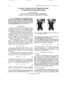
4.3 Rectangular plate with four openings As shown in Fig. 9, this rectangular plate with 4 openings, has 760 meshes. The numbers of medians considered as k={5 and 10}.The results are presented in Table 3 and the average convergence histories are depicted in Fig. 10.



241

Figure 9. The FE meshes of example 3 Table 3: Comparison of the statistical results for Example 3 Algorithm

ABC BBO HS TLBO

Initialization

Random k-means++ Random k-means++ Random k-means++ Random k-means++

Average k=5 4812.5 4815.6 4488.2 4492.5 4582.3 4582.5 4507.9 4513.5

k=10 3465.5 3475.6 2971.1 2962.9 3304.6 3296.3 3055.4 3064.9

Best k=5 4670 4694 4467 4467 4502 4482 4467 4467

k=10 3362 3372 2934 2934 3215 3202 2968 2959

Standard deviation k=5 k=10 63.9 47.4 67.6 48.2 65.4 20.1 50.2 31 45 33.3 62.4 51.2 39.7 41.4 61.3 36.5

CPU time (sec) k=5 k=10 18.4 19.5 17.8 18.9 9.1 9.8 9.1 9.8 8.9 9.5 9 9.7 19.6 20.2 19.1 19.5

a b Figure 10. The average convergence histories of Example 3 obtained by different methods: (a) k=5. (b) k=10



242

As presented in Table 3, the BBO outperformed other methods in terms of average cost and best cost, while HS completed the optimization process in lower CPU time. According to Fig. 10 the convergence speed of the BBO is more than other compared methods. The optimal domains and medians of both cases are plotted in Fig. 11.

a b Figure 11. A FEM divided into k subdomains using the BBO algorithm: (a) k=5. (b) k=10

4.4 Perforated circular plate A circular plate is considered as shown in Fig. 12. This FEM contains 1152 meshes and the number of subdomains are set to k= {4 and 5}. The statistical results are provided in Table 4 and convergence curves are plotted in Fig. 13.

Figure 12. The FE meshes of a circular plate



Algorithm ABC BBO HS TLBO

Table 4: Comparison of the statistical results for example 4 Initialization Average Best Standard deviation k=5 k=10 k=5 k=10 k=5 k=10 Random 7562.6 5623.1 7283 5486 100.5 60.6 k-means++ 7589.7 5651.5 7325 5549 98.3 54.2 Random 7271 5261.6 7230 5210 58.1 35.5 k-means++ 7312.1 5257.3 7230 5188 107.7 36.5 Random 7540.2 5605.6 7413 5419 71 55.1 k-means++ 7521.6 5602.6 7296 5489 95.1 49.3 Random 41 7257.6 5281.1 7230 5210 26.1 k-means++ 7273 5292.2 7230 5207 35.2 50.7

243

CPU time (sec) k=5 k=10 28.1 29.7 29.1 31.1 13.5 15.2 13.4 15.2 13.2 14.8 14.3 16.9 26.8 30.6 27.4 30

a b Figure 13. The average convergence histories of circular plate obtained by different methods: (a) k=5. (b) k=10

In this case, the best results are obtained by BBO and TLBO, while consumed time by HS is slightly lower than the BBO. Convergence curves also show better convergence of the BBO and TLBO. The optimal solutions are illustrated in Fig. 14.

a b Figure 14. A FEM divided into k subdomains using the BBO algorithm: (a) k=5. (b) k=10

244



5. CONCLUSION Four well-known metaheuristics are applied to optimal domain decomposition of FE models with different topology and number of meshes. According to results, BBO algorithm has generally performed better in most cases. According to Fig. 15(a) BBO algorithm has better performance, when is initialized by k-means++, except in standard deviation item. However by considering all algorithms, both initializations are almost equal and the only advantage of above initialization approach is lower required time to optimize, as depicted in Fig. 15(b). After BBO, the TLBO has obtained good convergence rate, average and minimum results, also, HS algorithm has consumed little time for completing the optimization procedure. Finally, this study suggests the implementation of BBO for the domain decomposition of finite elements due to the superiority of the results obtained by this method.

a b Figure 15. Outperforming percent of different initialization approaches: (a) in BBO algorithm. (b) by considering all algorithm

REFERENCES 1. Michael R. Garey, David S. Johnson. Computers and Intractability: A Guide to the Theory of NP-Completeness, W.H. Freeman, ISBN 0-7167-1045-5, 1979. 2. Farhat C, A simple and efficient automatic fem domain decomposer, Comput Struct 1988; 28: 579-602. 3. Farhat C, Lesoinne M. Automatic partitioning of unstructured meshes for the parallel solution of problems in computational mechanics, Int J Numer Meth Eng 1993; 36: 745-64. 4. Khan A, Topping B. Subdomain generation for parallel finite element analysis, Comput Syst Eng 1993; 4: 473-88.



245

5. Khan A, Topping B. Parallel adaptive mesh generation, Comput Syst Eng 1991; 2: 75-101. 6. Kaveh A, Roosta G. An algorithm for partitioning of finite element meshes, Adv Eng Softw 1999; 30: 857-65. 7. Kaveh A. Computational Structural Analysis and Finite Element Methods, Springer Science & Business Media, Switzerland, 2013. 8. Kaveh A, Sharafi P. Ant colony optimization for finding medians of weighted graphs, Eng Comput 2008, 25: 102-20. 9. Kaveh A, Shojaee S. Optimal domain decomposition via p-median methodology using ACO and hybrid ACGA, Finite Elem Anal Des 2008, 44: 505-12. 10. Kaveh A, Mahdavi VR. Optimal domain decomposition using the global sensitivity analysis based metaheuristic algorithm, Scientia Iranica; Trans A, Civil Eng, 2017, Published Online. 11. Kaveh A, Mahdavi VR. Optimal domain decomposition using colliding bodies optimization and k-median method, Finite Elem Anal Des 2015; 98: 41-9. 12. Kaveh A, Dadras A. Structural damage identification using an enhanced thermal exchange optimization algorithm. Eng Optim 2017; Published online. 13. Geem ZW, Kim JH, Loganathan G. A new heuristic optimization algorithm: harmony search. Simul 2001; 76(2): 60-8. 14. Kaveh A. Dadras A. A guided tabu search for profile optimization of finite element models. Int J Optim Civil Eng 2017; 7(4): 527-37. 15. Kaveh A, Dadras A. A novel meta-heuristic optimization algorithm: Thermal exchange optimization. Adv Eng Softw 2017, Published online. 16. Alp O, Erkut E, Drezner Z. An efficient genetic algorithm for the p-median problem, Annals Oper Res 2003; 122: 21-42. 17. Estivill-Castro V, Torres-Velázquez R. Hybrid genetic algorithm for solving the p-median problem, Simul Evol Learn 1999; 18-25. 18. McKendall AR, Shang J. Hybrid ant systems for the dynamic facility layout problem, Comput Operat Res 2006; 33: 790-803. 19. Maniezzo V, Mingozzi A, Baldacci R. A bionomic approach to the capacitated p-median problem, J Heurist 1998; 4: 263-80. 20. Levanova TyV, Loresh M. Algorithms of ant system and simulated annealing for the pmedian problem, Automat Remote Control 2004; 65: 431-8. 21. Kaveh, A., Advances in Metaheuristic Algorithms for Optimal Design of Structures. 2nd edition, Springer, Switzerland, 2017 22. Karaboga D, Basturk B. A powerful and efficient algorithm for numerical function optimization: artificial bee colony (ABC) algorithm, J Global Optim 2007; 39: 459-71. 23. Simon D, Biogeography-based optimization, IEEE Trans Evol Comput 2008; 12: 702-13. 24. Rao RV, Savsani VJ, Vakharia D. Teaching-learning-based optimization: a novel method for constrained mechanical design optimization problems, Comput-Aided Des 2011; 43: 303-15. 25. Arthur D, Vassilvitskii S. k-means++: The advantages of careful seeding, in: Proceedings of the Eighteenth Annual ACM-SIAM symposium on Discrete algorithms: Society for Industrial and Applied Mathematics 2007; pp. 1027-1035. 26. Kaveh A, Roosta GR. Comparative study of finite element nodal ordering methods, Eng Struct 1998; 20(1-2): 86-96 27. Kaveh A. Structural Mechanics: Graph and Matrix Methods, in: Research Studies Press Ltd, 2004. 28. Lloyd S. Least squares quantization in PCM, IEEE Trans Inform Theory 1982; 28: 129-37.


246


29. Kaveh A. Applications of Metaheuristic Optimization Algorithms in Civil Engineering: Springer, Switzerland, 2017. 30. Talbi EG. Metaheuristics: From Design to Implementation: John Wiley & Sons, Vol. 74, 2009. 31. Karaboga D. An idea based on honey bee swarm for numerical optimization, in: Technical report-tr06, Erciyes University, Engineering Faculty, Computer Engineering Department, 2005. 32. Sonmez M, Discrete optimum design of truss structures using artificial bee colony algorithm, Struct Multidiscip Optim 43 2011 85-97. 33. Saka MP, Aydogdu I, Hasancebi O, Geem ZW, Harmony Search Algorithms in Structural Engineering, in: Yang XS, Koziel S (Eds.) Comput Optim Appl Eng Indust 2011; pp. 145182, Berlin, Heidelberg: Springer Berlin Heidelberg. 34. Kaveh A, Mahdavi V. Colliding bodies optimization: A novel meta-heuristic method, Comput Struct 2014; 139: 18-27.

optimal decomposition of finite element meshes via k-median ...

optimal decomposition of finite element meshes via k-median ...

Suggest Documents

on moving finite element meshes - IEEE Xplore

finite element decomposition of the human neocortex

direct modification of finite element meshes preserving group ... - LSIS

Generating accurate finite element meshes for the forward model of ...

effects of warping finite element meshes for the forward ... - CiteSeerX

Quadrilateral Meshes for Finite Element-Based Image Registration

Nonstandard finite element de Rham complexes on cubical meshes

Algebraic Surface Design and Finite Element Meshes - Purdue e-Pubs

Quadrilateral Meshes for Finite Element-Based Image Registration

Finite element computations on quadtree meshes: strain smoothing ...

A numbering algorithm for finite element on extruded meshes which

Generating Anatomically Accurate Finite Element Meshes for Electrical ...

Domain Decomposition Method for a Finite Element ... - AndrÃ© Gaul

Optimal convergence analysis of an immersed interface finite element

Adaptive Finite Element Methods for Optimal Control of ... - CiteSeerX

Optimal Control of a Finite-Element Limited-Area ... - Semantic Scholar

Optimal Convergence Rates of Moving Finite Element Methods for ...

Optimal convergence rates of hp mortar finite element methods for ...

Finite Element Analysis and Optimal Design of ... - ATLANTIS PRESS

Finite Element Approximation of 2D Parabolic Optimal Design Problems

A Finite Element Solution of the Beam Equation via MATLAB

A Finite Element Solution of the Beam Equation via MATLAB

Finite Element modeling of hard turning process via a

Stability in Queueing Networks via the Finite Decomposition Property