ing optimal experimental designs subject to cost constraints in simulta- neous equations ..... controlled variation in the prices of gas and repairs, Pg and Pr, using its service station outlets as a ..... Bazi A free computer pro- gram for proportional ...
Optimal designs subject to cost constraints in simultaneous equations models ´ V´ıctor Casero–Alonso and Jesus ´ Lopez–Fidalgo Department of Mathematics, University of Castilla–La Mancha, Ciudad Real, Spain. Summary. A procedure based on a multiplicative algorithm for computing optimal experimental designs subject to cost constraints in simultaneous equations models is presented. A convex criterion function based on a usual criterion function and an appropriate cost function is considered. A specific L–optimal design problem and a numerical example are taken from Conlisk (1979) to compare the procedure. The problem would need integer non linear programming to obtain exact designs. To avoid this he solves a continuous non linear programming problem and then he rounds–off the number of replicates of each experiment. The procedure provided in this paper reduces dramatically the computational efforts computing optimal approximate designs. It is based on a specific formulation of the asymptotic covariance matrix of the full–information maximum likelihood estimators, which simplifies the calculations. The design obtained for estimating the structural parameters of the numerical example by this procedure is not only easier to compute, but also more efficient than the design provided by Conlisk. Keywords:
Approximate design, Cost constraints, Exact design,
L–optimal design, Multiplicative algorithm, Simultaneous equations, Structural equations.
2
1.
´ V´ıctor Casero–Alonso and Jesus ´ Lopez–Fidalgo
Introduction
Optimal experimental designs when constraints are imposed have been considered in the literature widely (see e.g. Cook and Fedorov, 1995). In this paper the problem is focused on the total cost of the experiment. A scalar coefficient will tune the compromise between information and cost (benefit). The novelty is to consider this approach for a model of simultaneous equations. These models are very common in the economics literature among other areas. As far as the authors know the first who considered the problem of designing experiments for simultaneous equations models was Conlisk (1979). For him the natural approach, as in standard regression, is to minimize a scalar function of the covariance matrix of the estimated structural coefficients of the simultaneous equations model. He proposed a design objective function based either on the three–stage least squares (3SLS) estimators introduced by Zellner and Theil (1962), or on the full–information maximum likelihood (FIML) estimators. These are the most commonly used estimation procedures for these models. The FIML method is computationally expensive as many authors pointed out. But the 3SLS method needs the reduced–form of the simultaneous equations model, that is, the set of equations that expresses each endogenous variable solely in terms of the exogenous variables. In the structural form of the model each endogenous variable is specified as a regression over the exogenous and the endogenous variables. Rothenberg and Leenders (1964) gave an explicit expression for asymptotic covariance matrix of FIML estimators which is equivalent to the asymptotic covariance matrix of 3SLS estimators of the structural coefficients, assuming the normal distribution for the disturbances. Finally, Conlisk
Optimal designs subject to cost constraints in simultaneous equations models
pointed out that the nonlinear restrictions on the reduced–form coefficients implied by the structural model causes the design criteria to be functions of unknown parameters. For handling these nonlinear restrictions Papakyriazis (1986) suggested the combination of sequential estimation and design control strategies. There is no much literature about optimal design for simultaneous equations models. Casero–Alonso and L´opez–Fidalgo (2014) proposed an alternative approach using triangular simultaneous equations models to the optimal experimental design problem for a linear regression model with explanatory variables that are not subject to the control of the practitioner. They obtained optimal designs for this model. Here it is extended to a problem with cost constraints. Casero–Alonso and L´opez– Fidalgo (2014) calculated the Information Matrix as the expected value of the partial derivative of the loglikelihood function with respect to the parameters of a triangular model, FIML method. In this paper the direct expression of the asymptotic covariance matrix of the FIML estimators provided by Rothenberg and Leenders (1964) is used for a more general model and an efficient iterative procedure is proposed to find optimal designs. In order to compute optimal designs we consider a multiplicative algorithm based on a convex criterion function. The multiplicative algorithm (e.g. Torsney and Mart´ın–Mart´ın, 2009) is used to update simultaneously all weights of the design points, step by step. A modification of the weighted average of an optimality criteria and a cost function (Pronzato, 2010) is considered in order to fit better the procedure. Cook and Wong (1994) showed that constrained and compound optimal designs approaches to handling multiple objectives are equivalent. This approach is based on approximate designs. But an exact design
3
4
´ V´ıctor Casero–Alonso and Jesus ´ Lopez–Fidalgo
is the final objective. The difference is not trivial. An exact design will be a collection of points x1 , ..., xn for a fixed number of experiments, n. Some of these points may be repeated. A discrete probability can be defined from it assigning the proportion of repetitions of each point in the design. Extending this, Kiefer (1959) defined an approximate design as a probability measure on χ, say ξ. This definition provides a framework for constructing optimal approximate designs and for discussing various optimality properties of designs in linear models using tools from convex analysis. The organization of this paper is as follows. In Section 2 the simultaneous equations model and the optimal experimental design problem in that model subject to a cost constraint is defined. In Section 3 a procedure to solve optimal design problems using a multiplicative algorithm, is presented. In Section 4 L–optimal designs subject to cost constraints are obtained in a couple of numerical examples. A discussion concludes this paper.
2.
Optimal experimental designs in simultaneous equations models
In this section a general problem of designing an optimum experiment for a simultaneous equations model subject to cost constraints is formulated. First the usual notation of simultaneous equations is introduced. Let us suppose a complete system of r linear stochastic structural equations in r jointly dependent variables and k predetermined explanatory variables, yi = Yi αi + Xi βi + ui = Zi δi + ui ,
i = 1, ..., r,
(1)
where yi is the n × 1 vector of observations of one of the endogenous
Optimal designs subject to cost constraints in simultaneous equations models
dependent variables, n is the number of experiments, Yi is the n × ri matrix of values formed by the ri ≤ r − 1 explanatory endogenous variables included in that equation, Xi is the n × ki matrix of values formed by the ki ≤ k explanatory exogenous variables included in that equation, αi and βi are ri × 1 and ki × 1 structural parameters vectors to be estimated, for the included endogenous and exogenous variables respectively, and ui is the n×1 vector of structural disturbances that have zero mean and are independent and homoscedastic across observations, that is with common covariance matrix, cov(u1h , ..., urh ) = Σ, h = 1, . . . , n. Let yi = Zi δi + ui where Zi = (Yi , Xi ) and δi = (αi , βi ). Furthermore, let us suppose that the reduced–form of the structural equations system exists, Y = XΠ + V , where Y is the matrix of endogenous variable observations, X is the matrix of values of the exogenous variables, Π is the coefficients matrix, and V is the reduced–form disturbances matrix. Let Yi = XΠi + Vi where Πi and Vi are submatrices of Π and V for that part of the reduced–form corresponding to Yi . As mentioned above the most common methods to estimate the structural coefficients δ = (α1 , β1 , . . . , αr , βr )T of (1) are 3SLS, three–stage least squares, and FIML, full–information maximum likelihood. The 3SLS method (Zellner and Theil, 1962) estimates the coefficients in three stages. The first serves to estimate the moment matrix of the reduced– form disturbances. In the second stage the coefficients of one single structural equation are estimated. Using the two–stage least squares estimated moment matrix of the structural disturbances, all coefficients of the entire system are estimated simultaneously in the third stage. The asymptotic covariance matrix of 3SLS or FIML estimators of structural coefficients δ of (1) assuming the normal distribution for the
5
´ V´ıctor Casero–Alonso and Jesus ´ Lopez–Fidalgo
6
disturbances is � � 2 ? ��−1 � �−1 ∂ L ˆ plim (cov δ) = −n lim E = H T (Σ−1 ⊗ (X T X))H , T n→∞ ∂δ∂δ (2) where plim indicates the probability limit, L? is the ‘concentrated’ likelihood function (see Rothenberg and Leenders, 1964), ⊗ represents the Kronecker product of matrices and H 0 1 .. H= . 0 Hr
,
(3)
where Hi = (Πi , Ji ) and Ji is defined by Xi = XJi , the matrix of unit vectors that select from X the exogenous variables of the ith equation.
2.1.
A specific design problem
Once the model is defined a set of specifications to state the optimal experimental design problem is needed: the design space X , the experimenter’s objective function and the cost constraints, if any. Although the design space could be continuous, the search is usually restricted to finite designs (Karlin and Studden, 1966). Regarding the objective function, any of the classical criteria of optimal experimental design, as D-optimality, A–optimality, c–optimality..., could be considered. To illustrate the procedure introduced in this paper, a specific L– optimal design problem is considered. A L–optimal design ξ ? is a design that minimizes the trace of LM (ξ)−1 (Atwood, 1976), where M (ξ) is the Information Matrix associated to an approximate design ξ and L is a definite positive user–selected matrix. L is chosen to reflect the researcher’s interest in the study. In the example considered here, the experimenter’s objective function is the sum of estimation error vari-
Optimal designs subject to cost constraints in simultaneous equations models
ances for predicting yi , i = 1, ..., r, that is, the predicted values of the left–hand variable of each structural equation, evaluated at each of the points of the finite design space X = {x1 , . . . , xm }. The cost constraint P is m i=1 cj nj ≤ C, where cj is the cost of taking one observation at xj , nj is the number of times xj appears in the final design and C is the total budget of the experiment. Putting all this together, the specific L–optimal experimental design problem can be stated as −1 X X min tr H T (Ir ⊗ xTj xj )H H T Σ−1 ⊗ nj xTj xj H n1 ,...,nm j j X s.t. nj cj ≤ C and n1 ≥ 0, . . . , nm ≥ 0, j
(4) where Ir is the identity matrix of order r. As Conlisk (1979) pointed out, though the nj must be integers (exact design), the usual procedure is to approximate by solving the continuous nonlinear programming problem and rounding–off the optimal values of nj .
3.
An efficient iterative procedure
In this section a procedure to solve the experimental design problem in a simultaneous equations model subject to a cost constraint stated in (4) is established. It is an anternative to the computationally expensive continuous nonlinear programming problem. Given that X T X of (2) can be expressed as
P
j
nj xTj xj in (4), that
is, as a weighted sum of the information matrices of the support points, approximate designs may be used here. Then a multiplicative algorithm for approximate designs can be applied. At each step the weights of the design points, ξ(xj ), will be adjusted. Therefore, one of the advantages
7
8
´ V´ıctor Casero–Alonso and Jesus ´ Lopez–Fidalgo
of the procedure described below is the reduction in time of computation (see a comparison of computational times in Section 55). Problem (4) is equivalent to obtaining the optimal approximate design ξ ? that minimizes the convex criterion function (Cook and Wong, 1994) Φβ (ξ) = Φ(ξ) − βB(ξ),
(5)
where ξ is an approximate design, Φ is an optimality criterion function (usually a function of M −1 (ξ)), B(xj ) is an appropriate benefit function P based on the known cost function cj , B(ξ) = i ξ(xj )B(xj ) which is linear in ξ and β > 0 is a parameter to be tuned. Note that the sign minus previous to β is to obtain the maximum benefit/minimum cost. The General Equivalence Theorem, GET (Kiefer and Wolfowitz, 1959) says that ξ ? is Φβ –optimal if and only if ∂Φβ (ξ, 1xj ) = tr{∇Φ(ξ)[M (1xj )−M (ξ)]}−β[B(1xj )−B(ξ))] ≥ 0, j = 1, ..., m, where ∂Φ(ξ, ξ 0 ) is the directional derivative of Φ at ξ in the direction of ξ 0 , that is
Φ[(1 − ε)ξ + εξ 0 ] − Φ(ξ) ε→0 ε is the design concentrated at xj , i.e. with weight 1 at xj . ∂Φ(ξ, ξ 0 ) = lim+
and 1xj
Based on the GET a multiplicative algorithm is used (Torsney and Mart´ın–Mart´ın, 2009). For a specific value of β, at step s+1 the weights of the design are updated, ξ
(s+1)
(xj ) = ξ
With this formula
P
j
(s)
� βB(1xj ) − tr ∇Φ(ξ (s) )M (1xj ) � . (xj ) βB(ξ (s) ) − tr ∇Φ(ξ (s) )M (ξ (s) )
(6)
ξ (s+1) (xj ) = 1.
For setting a stopping rule, a lower bound of the efficiency of the new design ξ (s+1) is computed. Again it is based on the GET, and it depends on the sign of Φβ (ξ (s+1) ),
Optimal designs subject to cost constraints in simultaneous equations models
• If Φβ (ξ (s+1) ) > 0 then effΦβ [M (ξ (s+1) )] ≥ 1 + K, • If Φβ (ξ (s+1) ) < 0 then effΦβ [M (ξ (s+1) )] ≥ 1/(1 + K), where K = min ∂Φβ (ξ (s+1) , 1xj )/Φβ (ξ (s+1) ). xj
For computing the optimal design ξ ? for the criterion (5) the following procedure is established: (a) For each particular value of β an optimal approximate design is obtained numerically, ξ (β) = arg min Φβ (ξ) = arg min [Φ(ξ) − βB(ξ)] , ξ
ξ
using the multiplicative algorithm (6). � � (b) Let β ? = arg min Φ n(β) ξ (β) where n(β) = C/C(ξ (β) ) is the total β P number of experiments for each β, and C(ξ (β) ) = j ξ (β) (xj )cj . ?
?
(c) Finally n(β ) ξ (β ) (xj ) has to be rounded–off to integers, n?j , in such P P ? ? a way j n?j ≈ n(β ) and nj cj ≈ C. This procedure could be adapted to any design problem.
4.
An illustrative example
To compare the procedure described above with the continuous problem stated in (4) the numerical example of Conlisk (1979) is considered. First we take a simplified version to illustrate both approaches. Later the full version of the example is commented. Let us suppose that a major oil company decides to experiment with controlled variation in the prices of gas and repairs, Pg and Pr , using its service station outlets as a cross–section of observations. Three alternate values (0.93, 1, 1.07) for each price variable (in an appropriate normalized
9
10
´ V´ıctor Casero–Alonso and Jesus ´ Lopez–Fidalgo
form) are considered. This makes a full factorial design space of 32 experimental conditions: X = {x1 = (0.93, 0.93), x2 = (0.93, 1), x3 = (0.93, 1.07), x4 = (1, 0.93),
x5 = (1, 1),
x6 = (1, 1.07),
x7 = (1.07, 0.93), x8 = (1.07, 1), x9 = (1.07, 1.07)}. The goal is to estimate the coefficients of the demand model (structural equations) of quantities of gas and repairs sold, Qg and Qr , Q =α +β Q +α P +u , g 11 11 r 12 g 1 Qr = α21 + β22 Qg + α22 Pr + u2 . To solve the corresponding experimental design problem (4) we must supply nominal values for Σ, disturbance covariance matrix, and H, where H depends on Π via (3) and Π in turn depends on the structural coefficients αi and βi . This is because the nonlinear restrictions on the reduced–form coefficients Π implied by the structural model. The prior specifications needed for computing the optimal design are Q = 1.38 + 0.1Q − 0.5P + u , 0.1 0.06 g r g 1 . Σ= Qr = 0.39 + 0.8Qg − 0.2Pr + u2 , 0.06 0.1 With these values we obtain the reduced–form system after some algebra, and therefore the nominal values of Π1 and Π2 . Then the Hi matrices are
1.6239
1 0
H1 = −0.4348 0 1 −0.2174 0 0
,
1.5424
1 0
H2 = −0.5438 0 0 −0.0217 0 1
.
Finally, the cost of making one experiment at the jth experimental condition (service station) is defined by cj = 5 + 3673(Pg(j) − 1)2 + 2857(Pr(j) − 1)2 + 1633(Pg(j) − 1)(Pr(j) − 1),
Optimal designs subject to cost constraints in simultaneous equations models
11
in terms of percentages of profit lost by stations during the experiment
(Conlisk 1979). The nine rounded–off unit costs are cj = {45, 23, 29, 19, 5, 19, 29, 23, 45}. There is symmetry in the unit costs. The minimum unit cost value is in the ‘central’ experimental condition, that is at standard price levels Pg = Pr = 1. The maximum cost values are in the ‘initial’ and ‘final’ experimental conditions (Pg = Pr = 0.93 and Pg = Pr = 1.07, respectively). That is, deviations of standard price levels are cost–penalized (yield percent profit losses). The total budget of the experiment is specified as C = 6500, which is the lost of all profits of 65 stations. With these specifications we will find numerically the optimal structural design, that is the solution of the design problem (4). In other words, the optimal approximate design for estimating the structural parameters of the simultaneous equations model subject to a cost constraint. There is not a unique global minimum, it depends on the starting point of the search. To illustrate the situation we consider three cases: • Case 1. Initial values of nj = 1, j = 1, ..., m. • Case 2. Initial values of nj = nmax /2, where nmax = arg max{nj |nj cj = j j 6500}, j = 1, ..., m. • Case 3. Initial values of nj = nmax − 1. j The optimal exact (rounded–off) designs obtained are presented in Table 1. Observe that when the initial values increase the nj of the odd design points decrease whereas the nj of the even points increase. Moreover, the ‘central’ design point receives the highest number of experiments. The total number of experiments varies from 332 in Case 2 to 335 in Case 3. For Case 1 is 333. For the three cases the value of the objective function (4) for the approximate design is 0.020973. If the optimal exact designs
12
´ V´ıctor Casero–Alonso and Jesus ´ Lopez–Fidalgo
Table 1. Optimal exact designs for estimating the structural parameters of the numerical exam
of Table 1 are considered the values of the objective function for Cases 1, 2 and 3 are 0.0211127, 0.021129 and 0.0209315 respectively. The later value is lower than the value for the optimal approximate design. The full version of the example considers other controlled variables, the dummies Dg and Dr , describing whether or not trading stamps are offered with gas and repair sales respectively. Then, the demand model is:
Q =α +β Q +α P +α D +u , g 11 11 r 12 g 13 g 1 Qr = α21 + β22 Qg + α22 Pr + α23 Dr + u2 . In this case, the design space X is 4–dimensional, (Pg , Pr , Dg , Dr )
with values 0 or 1 for Dg and Dr . This yields 32 × 22 = 36 experimental possible conditions: X = {x1 = (0.93, 0.93, 0, 0), x2 = (0.93, 0.93, 0, 1), x3 = (0.93, 0.93, 1, 0), x4 = (0.93, 0.93, 1, 1), x5 = (0.93, 1, 0, 0), . . . , x36 = (1.07, 1.07, 1, 1)}. The prior specifications of α13 and α23 are 0.04 and 0.02 respectively. And the cost of the jth experimental condition, service station, includes (j)
now the term 5(1 − Dg ) to penalize the absence of trading stamps of gas. There is no term to penalize presence/absence of trading stamps of repairs. Therefore each couple of experimental conditions (Pg , Pr , Dg , 0) and (Pg , Pr , Dg , 1) have the same unit cost. The rounded–off unit costs
Optimal designs subject to cost constraints in simultaneous equations models
13
Table 2. Rounded–off unit costs
are shown in Table 2. As in the simplified case, there is symmetry in the unit costs. The ‘central’ experimental conditions are the cheapest and the ‘extremes’ (Pg and Pr 6= 1) the most expensive ones. The optimal structural design for this case, provided by Conlisk (1979), is presented in Table 3. This exact design sums up to 529 experiments with a total cost of 6471. We were not able to compute this design directly. But, we have obtained approximate designs similar to the Conlisk design but with a lower value of the objective function (4). This means that the rounding–off procedure is an important issue (see Section 55). Now the optimal design with the procedure described in Section 33 for the numerical example is obtained. In order to apply it, a criterion function Φ(ξ), the benefit function B(ξ) and the values of the parameter β have to be selected. As described in Section 2.12.1 the criterion function considered is L– optimality: ΦL [M (ξ)] = tr[LM −1 (ξ)]. Then ∇ΦL [M (ξ)] = −M −1 (ξ)LM −1 (ξ)
14
´ V´ıctor Casero–Alonso and Jesus ´ Lopez–Fidalgo
Table 3. Optimal designs for estimating the structural parameters
for nonsingular information matrices. From (2) the FIM is X M (ξ) = H T Σ−1 ⊗ ξj xTj xj H j
with ξj = ξ(xj ) (such that
P
j ξj
P = 1). From (4) L = H T (I⊗ j xTj xj )H,
which is a positive definite matrix of the same dimension as M (ξ). P Let the benefit function be B(ξ) = j ξ(xj )B(xj ) where B(xj ) = 1/cj . The parameter β depends on the problem considered. For the simplified example the values of β are taken from the interval [0, 500]. Then, the steps of the procedure are applied as describeb in Section 33. First, for each β the approximate design reaching an efficiency of 99.9% is considered as optimal. The expression (6) for the step of the multiplicative algorithm in this case of L–optimality is � βB(xj ) − tr −M −1 (ξ (s) )LM −1 (ξ (s) )M (1xj ) (s+1) (s) � . P ξ (xj ) = ξ (xj ) β j ξ (s) (xj )B(xj ) − tr −M −1 (ξ (s) )L h i Among all β we choose β ? = arg min ΦL M (n(β) ξ (β) ) . Finally the opβ
timal exact design is obtained by rounding–off the optimal approximate
Optimal designs subject to cost constraints in simultaneous equations models
15
FLHΞL
nΒ 600
0.025
500
0.024
400
0.023
300
0.022
100
200
300
400
500
Β 100
200
300
400
500
Β
Fig. 1. Values of total number of experiments n(β) and criterion function ΦL (ξ) for different values of β parameter.
design of n(β
?
)
experiments.
In the simplified example β ? = 66.875 (see Figure 1, right) and the optimal exact design is presented as P in Table 1. For the approximate � � ? ? ? design of size n(β ) = 332.08, ΦL M (n(β ) ξ (β ) ) = 0.021223, and for the exact design 0.021222 (slightly better). For the full example the values of β are taken from the interval [0, 2000]. Then β ? = 586.5 and the optimal exact design is presented as P in Table 3. This design sums up to 446 experiments, 16% less than Conlisk exact design, which sums up to 529 experiments but the cost is � � ? ? about the same. In this example, ΦL M (n(β ) ξ (β ) ) = 0.0907064 for the approximate design and 0.091391 for the exact design. Tables 1 and 3 show big differences between the designs obtained through the two approaches. In the designs obtained with the procedure of Section 33 there are many 0’s, 4 of 9 in the simplified example, specifically at the even support points, and 26 of 36 in the full example. That is, for both examples the designs are concentrated at the ‘extremes’ and the central support points, as usual in standard regression. Although the different values, both approaches allocate the highest values of nj in
16
´ V´ıctor Casero–Alonso and Jesus ´ Lopez–Fidalgo
the central design points, the cheapest ones.
5.
Discussion
There are two main advantages of the procedure proposed in this paper. On the one hand, it saves time of computations. The design problem (4) and the alternative procedure have been implemented in M athematica. The time for obtaining any of the Cases 1, 2 or 3 are around 60 seconds, whereas our procedure needs only about 6 seconds. This point is crucial when the number of points increases. As a matter of fact the example of Conlisk (1979) considered 36 experimental conditions (points) (see Section 44). On the other hand, the designs obtained with our procedure have much larger efficiencies. To compare the designs we compute the relative L–efficiency of a design ξ with respect to another design ξ 0 of reference: effL (ξ, ξ 0 ) =
ΦL [M (ξ 0 )] , ΦL [M (ξ)]
where exact designs with integers nj , j = 1, ..., m are considered. Due to the consideration of these exact designs the magnitudes of information matrices vary depending on the sample size. The relative L–efficiency of the approximate design of 9 support points obtained with the procedure with respect to the Cases 1, 2 or 3 are 98,8%. If exact designs are considered the efficiency drops to 98,6% in the worst case. On the other hand, the exact design of 36 support points obtained with the alternative procedure is 26.6% more efficient than the structural design provided by Conlisk. Note that both designs are L–optimal restricted, both obtained for the same total cost not to the same total number of experiments. The advantages just mentioned are based on two points. On the one hand, the use of an efficient multiplicative algorithm. On the other hand
Optimal designs subject to cost constraints in simultaneous equations models
a convenient definition of the covariance matrix of the estimators of the structural parameters of the model. Moreover, the procedure could be adapted to any design problem. Another issue is the consideration of approximate designs when the problem considered requires an exact design. The Conlisk approach and our procedure solve the problem using approximate designs, which must be rounded–off. In our procedure the usual rounding–off of the values obtained is taken. But there are many rounding–off methods to be applied to an optimal approximate design (see Imhof, L´opez–Fidalgo and Wong, 2001 for a list). We have applied the rounding–off methods included in the software BAZI to the approximate solutions obtained. There are nine apportionment methods implemented in BAZI (Maier and Pukelsheim, 2007). From divisor methods, with rounding down (Jefferson/D’Hont/Hagenback–Bischoff), rounding up (Adams) or standard rounding (Webster/Sainte–Lagu¨e/Schepers) to quota methods: Hare–quota method with residual fit by greatest remainders (Hamilton/Hare/Niemeyer) and Droop–quota method with residual fit by greatest remainders. The rounded–off designs obtained with BAZI could be compared, if they are different. Therefore, the last step will be to choose the best one with respect to the criteria considered. For example, for the structural design of 36 support points the Hare–quota method provides an allocation that attains a lower ΦL (ξ) than the standard rounded–off solution of the procedure. The last one is another solution provided by BAZI, the apportionment obtained with the divisor method with standard rounding. The differences between the Hare–quota design and the rounded–off design are in two design points. In Pg = Pr = Dg = Dr = 1, where Hare–quota method allocates one experiment less than the rounding–off procedure, it goes from
17
18
´ V´ıctor Casero–Alonso and Jesus ´ Lopez–Fidalgo
166 to 165 experiments. This experiment ‘shifts’ to the design point Pg = Pr = 1.07; Dg = Dr = 0 where Hare–quota method allocates 27 experiments while the standard rounding–off procedure assigns 26 experiments.
Acknowledgments This work has been supported by Ministerio de Educaci´on y Ciencia and Fondos FEDER MTM2010–20774–C03–01 and Junta de Comunidades de Castilla la Mancha PEII10–0291–1850.
References Atwood, C. L. (1976). Convergent design sequences, for sufficiently regular optimality criteria. The Annals of Statistics. 4 (6), 1124– 1138. BAZI. Berechnung von Anzahlen mit Zuteilungsmethoden im Internet / Calculation of Allocations by Apportionment Methods in the Internet. http://www.uni-augsburg.de/bazi/ Casero–Alonso, V. and L´ opez–Fidalgo, J. (2014). Experimental Designs in Triangular Simultaneous Equations Models. Statistical Papers. (In press) DOI: 10.1007/s00362–014–0581–y Conlisk, J. (1979). Design for simultaneous equations. Journal of Econometrics. 11 (1), 63–76. Cook, D. and Fedorov, V. (1995). Constrained optimization of experimental design. Statistics. 26 (2), 129–178.
Optimal designs subject to cost constraints in simultaneous equations models
Cook, R.D. and Wong, W.K. (1994). On the equivalence of constrained and compound optimal designs. Journal of the American Statistical Association. 89 (426), 687–692. Imhof, L., L´ opez–Fidalgo, J. and Wong, W. K. (2001). Efficiencies of rounded optimal approximate designs for small samples. Statistica Neerlandica. 55, 301–315. Karlin, S. and Studden, W. (1966). Optimal experimental designs. The annals of mathematical statistics. 37, 783–810. Kiefer, J. (1959). Optimum experimental designs. Journal of the Royal Statistical Society, Series B. 21, 272–319. Kiefer, J., and Wolfowitz, J. (1959). Optimum design in regression problems. The Annals of Mathematical Statistics. 30, 271–294. Maier, S., and Pukelsheim, F. (2007). Bazi A free computer program for proportional representation apportionment. Preprint Nr. 42/2007. Institut f¨ ur Mathematik, Universit¨ at Augsburg. http://opus.bibliothek.uni-augsburg.de/volltexte/2007/711/ Papakyriazis, P.A. (1986). Adaptive optimal estimation control strategies for systems of simultaneous equations. Mathematical Modelling. 7, 241–257. Pronzato, L. (2010). Penalized optimal designs for dose–finding. Journal of Statistical Planning and Inference. 140, 283–296. Rothenberg, T.J. and Leenders, C.T. (1964). Efficient estimation of simultaneous equations systems. Econometrica. 32, 57–76.
19
20
´ V´ıctor Casero–Alonso and Jesus ´ Lopez–Fidalgo
Torsney, B. and Mart´ın–Mart´ın, R. (2009). Multiplicative algorithms for computing optimum designs. Journal of Statistical Planning and Inference. 139, 3947–3961. Zellner, A. and Theil H. (1962). Three–Stage least squares: simultaneous estimation of simultaneous equations. Econometrica. 30, 54–78.