Fast Control of Linear Systems Subject to Input Constraints

P. Tomas Larsson A. Galip Ulsoy Department of Mechanical Engineering and Applied Mechanics, University of Michigan, Ann Arbor, MI 48109-2125

1

Fast Control of Linear Systems Subject to Input Constraints Efficient design of high performance automatic control systems is extremely important for high technology systems. To get the best hardware cost-to-performance ratio, it is desirable to design a controller that takes full advantage of actuator capabilities, but this can lead to nonlinear behavior due to actuator saturation. The saturation nonlinearities in the system may have severe effects on system performance due to, for example, integrator windup. In this paper, a new design method is presented based on Lyapunov stability theory. By incorporating the actuator constraints directly in the design method, better utilization of the available control effort can be ensured in achieving desired system behavior. 关S0022-0434共00兲01801-3兴

Introduction

Every physical control system has some kind of actuator limitation or nonlinearity 共e.g., a motor can only supply limited torque and limited power兲. The actuator limitation ultimately limits the achievable closed-loop performance. Often, actuator constraints impose more severe performance limitations than other sources such as modeling uncertainties 关1兴. The effects of amplitude saturation have been extensively studied for decades, but it is not the only type of actuator saturation. Recently, increasing work has been done on the control of systems where the output rate of change of the actuator is limited 共e.g., 关2–4兴.兲 Power saturation depends on the product of two states 共e.g., voltage and current兲. Other constraints are internal to the plant. A plant state variable could, for example, be limited for safety reasons. The design method presented in this paper deals with the design of linear systems with input amplitude saturation. However, it can be extended to handle other types of constraints. The traditional design approach for systems with amplitude saturation has two-steps: A linear controller is designed first, ignoring the effects of actuator saturation, and then an ad hoc antiwindup 共AW兲 scheme is designed to reduce the problems that arise due to saturation nonlinearities. Since the constraints are not considered in the linear design it may not take full advantage of the available actuator capacity. Since the most severe wind-up problems often come from integral control, that is where much attention has been focused. See, e.g., the research on proportionalintegral-derivative 共PID兲 controllers in 关5–9兴. Another approach is to use guaranteed domains of attraction 共GDA兲 共invariant sets兲 to design a reference governor that restricts the reference signal to avoid saturation, see 关10兴. See also 关11兴, which uses GDA:s to avoid saturation by switching between increasingly ‘‘faster’’ controllers as the states approaches the set point. The design procedure presented in this paper can be applied to both full-state feedback and full-state feedback plus integral control for single-input single-output 共SISO兲 systems. When integral control is used, a simple AW scheme is added to improve system performance. First, the general design concept will be described. Second, several design examples are presented. They include simulation and experimental results that support the design approach. Additional examples that support the feasibility of the design method can be found in 关12兴. The ideas presented in this paper are closely related to work presented in 关13兴 and 关14兴, where the goal is to design a saturating controller that fully utilizes available control effort while optimizContributed by the Dynamic Systems and Control Division for publication in the JOURNAL OF DYNAMIC SYSTEMS, MEASUREMENT, AND CONTROL. Manuscript received by the Dynamic Systems and Control Division July 14, 1998. Associate Technical Editor: T. R. Kurfess.

18 Õ Vol. 122, MARCH 2000

ing performance. See 关15兴 for a method that results in a guaranteed cost in the presence of saturation. The design method presented in this paper differs in that the emphasis is on achieving a desired linear behavior, instead of robustness to saturation.

2

Assumptions The plant is given by the discrete-time system x共 t⫹1 兲 ⫽Ax共 t 兲 ⫹Bsat共 u 共 t 兲兲 ,

(1)

y共 t 兲 ⫽C1 x共 t 兲 ,

(2)

z 共 t 兲 ⫽C2 x共 t 兲 ,

(3)

n

with state x苸R , controlled output z苸R, output measurement y苸Rn , and actuator output u苸R. The saturation function is defined by sat共 u 兲 ⫽

再

u,

if abs共 u 兲 ⭐u max

sign共 u 兲 u max ,

if abs共 u 兲 ⬎u max

(4)

It is assumed that u max , is known. C1 is the identity matrix so that full state feedback, u⫽⫺Kx⫽⫺Ky

(5)

can be used. The reference input is assumed to be zero. If C1 ⫽I, the design method can still be used by designing a state observer. See 关16兴 for a discussion on the effect of the design of the observer on the proposed design method.

3

The Design Concept

In most research on saturating control it is assumed that a good linear design already exists, and the emphasis is on finding a method to minimize the effect of the saturation element on the system performance. The emphasis here is different, in that there is no a priori linear design. The goal of the design is to come up with a linear controller that with saturation minimizes the settling time of the system. A key idea is the scaling of the linear design by a parameter ␤⬎0 which is chosen so that the system performance improves as ␤ increases. It was shown in 关17兴 how such a dependency on ␤ can be achieved using linear quadratic regulator 共LQR兲 design. To make things specific, let the performance be measured by the settling time and choose the scaling parameter by pole placement. Specifically, suppose ␤ is determined by the following procedure: 1 Define vector of complex pole locations pb that results in a desirable system behavior. 2 Introduce a real scalar scaling parameter ␤ such that the final

Copyright © 2000 by ASME

Transactions of the ASME

Fig. 1 Scaling of poles

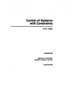
pole locations pc are defined by pc ⫽ ␤ pb 共see Fig. 1兲, or if discrete time control is used pc ⫽e ⫺ ␤ pb ⌬T , where ⌬T is the sampling time. This way of scaling maintains the damping of the poles, while changing the speed of the response. 3 Choose the feedback gains K( ␤ ), so that the closed loop poles are given by pc . This simple scaling idea is fine for many plants. Indeed, the performance cost 共settling time兲 will often be reduced as ␤ increases. In general, though, a more advanced form of scaling will be needed, such as the LQR based method in 关17兴. For example, if the plant transfer function has poorly placed zeros, the overshoot and hence the settling time might increase as ␤ is increased. The vector pb is assumed given and the nontrivial problem of how to choose it are not addressed here. The method of scaling is not critical to the design method as long as the performance cost is a monotone decreasing function of ␤. Clearly, if the control signal does not saturate, it is desirable to increase ␤. In the presence of saturation there will be a limit to the achievable performance, but that limit is generally not given by the onset of saturation. Figure 2 shows the 1 percent settling time, as a function of ␤, for the digital state feedback control of a double integrator plant: pb ⫽ 关 ⫺1,⫺1 兴 共i.e., a critically damped design兲, for an initial position displacement of 1, and a sampling time of 0.01 s. From Fig. 2 it is clear that the performance can be improved by increasing ␤ outside the interval (0,␤ lin) where the control does

not saturate. However, as ␤ is increased beyond ␤ opt the behavior of the system starts to deteriorate due to saturation effects. Similar results can be obtained using other performance measures, such as the integral of the squared error. The extent to which the behavior can be improved relative to the nonsaturating case are highly dependent on the dynamics of the open loop plant. The success of a controller designed in this manner may vary. The 1 percent settling time for the time optimal bang-bang control for the above example is 1.8 s, and, as can be seen from Fig. 2, it is possible to get quite close to that time by just using a linear feedback and letting it saturate. Of course, the time-optimal control reaches the set-point in finite time, whereas the linear saturating controller asymptotically approach the set-point. Similar conclusions have been drawn in 关18兴 for the proportional-derivative 共PD兲 control of second order systems. They show it is possible to increase the closed-loop bandwidth and decrease the root mean square 共RMS兲 error by choosing PD feedback gains so that the controller saturates. Since the design has been parameterized by a single design parameter ␤ it is easy to do a search over ␤ to find the optimal value for a particular initial condition 共or step input size兲. In general, it is desirable to have a good response for a set of initial conditions, not just one particular initial condition. In this case, it is natural to minimize the worst case settling time, i.e.,

␤ opt⫽arg min共 max t s 兲 , ␤

(6)

x 0 傺IC

where IC is the specified set of initial conditions. While the optimal solution to Eq. 共6兲 may be achieved numerically for systems of very low order by repeated simulation, it is generally intractable. Another disadvantage of trying to solve Eq. 共6兲 is that nothing is known about the robustness of the design. Another approach, which circumvents Eq. 共6兲 is to construct a guaranteed domain of attraction, ⍀ s ( ␤ ). The ‘‘size’’ of ⍀ s ( ␤ ) generally becomes smaller as ␤ increases. The idea is to maximize ␤ under the constraint that IC傺⍀ s ( ␤ ). The resulting value of ␤ is

␤ sat⫽ max ␤ .

(7)

IC傺⍀ 共 ␤ 兲

While it is generally true that ␤ sat is less than ␤ opt , solving for ␤ sat is numerically feasible and it can produce efficient designs. Moreover, designs can also be made robust to disturbances and parameter uncertainties 共see 关16兴兲. A method for constructing ellipsoidal GDA’s is described in the following section. Notice that as long as a monotone dependence between a scalar design parameter and a performance cost can be identified any linear design technique 共state space or frequency domain兲 can be used to do the scaling. In this paper, pole placement is used to perform the scaling for the initial examples, and LQR design is used to do the scaling for the experimental setup.

4

A Guaranteed Domain of Attraction

First, we state a theorem that for fixed K determines an ellipsoidal domain of attraction for the saturated feedback system determined by Eqs. 共1兲–共5兲. The proof depends on a simple application of the discrete-time Lyapunov equation. The proof for the continuous-time case can be obtained by using the continuoustime Lyapunov equation instead of the discrete time Lyapunov equation. Given an m⫻m, positive definite symmetric matrix P, and a feedback gain K that stabilizes the system x(t⫹1)⫽(A ⫺BK)x(t), let 0⬍ ␣ min⬍1, be a number such that the matrix inequality 共 A⫺ ␣ BK兲 T P共 A⫺ ␣ BK兲 ⫺P⬍⫺ ⑀ I

Fig. 2 Scaling design for PD control of a double integrator plant

Journal of Dynamic Systems, Measurement, and Control

(8)

is satisfied for all ␣ 苸 关 ␣ min,1兴 , for a fixed P, and for an arbitrarily small constant ⑀ ⬎0. Note that ␣ min will depend on K and P. A necessary condition for the existence of a matrix P that satisfies Eq. 共8兲 for all ␣ 苸 关 ␣ min,1兴 is that all the eigenvalues of the matrix A⫺ ␣ BK are placed inside the unit disk for ␣ 苸 关 ␣ min,1兴 . MARCH 2000, Vol. 122 Õ 19

Theorem 4.1. Define

␥ , 共 KP

⫺1

2 ⫺2 KT 兲 ⫺1 u max ␣ min

(9)

and ⍀ s 共 K,P兲 , 兵 x苸Rn 兩 xT Px⭐ ␥ 其

(10)

x共 t⫹1 兲 ⫽A⫺Bsat共 Kx共 t 兲兲

(11)

Then the system has an asymptotically stable equilibrium point at x⫽0 and ⍀ s is a guaranteed domain of attraction. Specifically, x(0)苸⍀ s implies x(t)苸⍀ s for all t⬎0 and x共 t 兲 →0 as t→⬁

(12)

Proof: First we show that x苸⍀ s implies sat(Kx)⫽ ␣ (x)Kx where ␣ min⭐␣(x)⭐1. It is clear that ␣共x兲⫽1 when 兩 Kx兩 ⭐u max and ␣共x兲 is minimum when 兩Kx兩, x苸⍀ s , is maximum. The condition ␣ min⭐␣(x) is achieved by choosing ␥ appropriately. The maxx苸⍀ s Kx exists since ⍀ s is compact. Moreover, a maximizing state x* must satisfy the multiplier rule for inequality constraints: ␭ⵜKx⫽ⵜ(xT Px⫺ ␥ ) at x⫽x*, ␭⭓0. Equivalently x* ⫽⫺(1/2␭)P⫺1 KT . Substituting x* ⫽⫺(1/2␭)P⫺1 KT into x* T Px* ⫽ ␥ and ␣ minKx* ⫽u max and solving for ␥ results in Eq. 共9兲. Now let V(x)⫽xT Px and form V 共 x共 t⫹1 兲兲 ⫽xT 共 t⫹1 兲 Px共 t⫹1 兲 .

(13)

Since x„0…苸⍀ s , ␣ (x„0…)⭓ ␣ min is guaranteed to hold. Consequently, the inequality in Eq. 共8兲 holds and V 共 x共 1 兲兲 ⭐V 共 x共 0 兲兲 ⫺ ⑀ 兩 x共 0 兲 兩 2 ⭐ ␥ .

(14)

Repeating the argument for increasing t shows that V 共 x共 t 兲兲 ⭐ ␥

᭙t⭓0.

(15)

Thus, x(t)苸⍀ s , t⭓0, also, V 共 x共 t⫹1 兲兲 ⫺V 共 x共 t 兲兲 ⭐⫺ ⑀ 兩 x共 t 兲 兩 2

᭙t⭓0.

(16)

Result 共12兲 is true if x(t)⫽0 for some t⭓0. Thus, suppose 兩 x(t) 兩 ⬎ ⑀ ᭙t⭓0. Since V(x(t)) is strictly decreasing, and bounded from below it has to converge to a limit, say V * . Using V 共 x共 t 兲兲 ⫺V 共 x共 t⫺1 兲兲 ⭓ ⑀ 兩 x共 t 兲 兩 2

᭙t⭓0

(17)

it follows that 兩 x(t) 兩 →0. 䊐 Theorem 4.1 is illustrated schematically for a second order example in Fig. 3. Theorem 4.1 does not say anything about how to obtain the matrix P. Any choice of P that satisfies Eq. 共8兲 for ␣ ⫽1 can be used; it then follows that there exists an ␣ min⬍1.

However, the ‘‘size’’ and ‘‘shape’’ of the GDA ⍀ s will depend on the choice of P. In the design procedure a search will be made to find a matrix P, that results in IC傺⍀ s . The stability result obtained in Theorem 4.1 is sufficient, but not necessary to guarantee asymptotic stability, and therefore the obtained GDA will be conservative. A similar method was used by 关11兴 to define domains of attraction, but they wanted to avoid saturation. In 关19兴 the use of higher order Lyapunov functions were investigated to obtain a less conservative estimate of the set for which it can be guaranteed that the controller will not saturate. In 关12兴 it was shown how the obtained GDA can be made robust to bounded input disturbances and parameter uncertainties that satisfies the matching condition. If the inequality in Eq. 共8兲 holds for all ␣ 苸(0,1兴 , then the system in Eq. 共11兲 is globally asymptotically stable 共GAS兲. This was used in 关20–22兴 to ensure global stability for systems with no right-hand poles or repeated poles on the imaginary axis. Since the GDA is bounded, there is more freedom in changing the feedback gains compared to when global stability is required. The method can also be applied to open-loop unstable systems. Different P will result in different values for ␣ min , and different ‘‘sizes’’ for the set ⍀ s . It is desirable to find a Lyapunov function that results in a sufficiently large ⍀ s , which in general means a small ␣ min 共see Eq. 共9兲兲. Satisfaction of the criterion IC傺⍀ s depends on K( ␤ ), and the matrix P. As discussed in Section 3 it is desirable to maximize ␤ to improve performance, while being able to guarantee stability. By defining

␣ min⫽

␣,

inf 共 A⫺ ␣ BK兲 T P共 A⫺ ␣ BK兲 ⫺P⬍⫺ ⑀ I

(18)

᭙ ␣ 苸 关 ␣ min,1兴

the problem of finding the ‘‘best’’ controller for a given P can be formulated as

␤ sat⫽

max IC傺⍀ s 共 P,K共 ␤ 兲兲

␤.

(19)

Thus, ⍀ s (P,K( ␤ )) replaces ⍀共␤兲 in Eq. 共7兲. Since ⍀ s is convex it follows that IC傺⍀ s ⇒coIC傺⍀ s . In addition, since ⍀ s is symmetric around the origin IC傺⍀ s ⇒co共IC艛⫺IC兲傺⍀ s , where ⫺IC⫽ 兵 x苸Rn 兩 ⫺x苸IC其 . Consequently, it is sufficient to define a set IC* consisting of a finite number of points, where IC* is chosen so that IC傺co共IC* 艛⫺IC* ). Then, IC* 傺⍀ s ⇒IC傺⍀ s will hold. This means that the condition in Eq. 共19兲 only has to be checked for a finite number of points, IC* , even if the set of initial conditions, IC, has an infinite number of possible initial conditions. A software that performs the design has been developed in Matlab. In the developed software a numerical search is performed to find the matrix P that results in the largest ␤ sat . The basic structure of the algorithm is described informally by the following five steps: 1 Choose an initial ␤. 2 Repeat steps 3–5 until ␤ is determined within a specified tolerance. 3 Search for a P that satisfies IC傺⍀ s (P,K( ␤ )). 4 If a P can be found such that IC傺⍀ s (P,K( ␤ )), then increase ␤ and go to 3. 5 If a P cannot be found such that IC傺⍀ s (P,K( ␤ )), then reduce ␤ and go to 3. The key step is step 3 where the P matrix is obtained. The P matrix is obtained by defining the function S 共 P, ␤ 兲 ⫽ ␥ 共 P,K共 ␤ 兲 ,u max兲 ⫺1 max xT Px.

(20)

x苸IC

Fig. 3 Two-dimensional example

20 Õ Vol. 122, MARCH 2000

When S(P, ␤ )⬍1 holds, it follows from Eq. 共10兲 that IC傺⍀ s (P,K( ␤ )) holds. Since any S(P, ␤ )⬍1 guarantees the stability, it is desirable to minimize S(P, ␤ ) with respect to P⫽PT ⬎0. Since S(P, ␤ ) is a well-defined objective function, any Transactions of the ASME

Table 1 Comparison of design methods, full state feedback

of a number of numerical optimization techniques can be used to minimize S(P, ␤ ) for a fixed ␤, and thereby find a P such that IC傺⍀ s 共 P,K共 ␤ 兲兲 .

(21)

There is no guarantee that there exists a pair P, ␤ such that Eq. 共21兲 is satisfied for an open-loop unstable system, in fact, if a system is open-loop unstable and the input control is bounded, there exists initial states from which it is impossible to stabilize the system. To reduce the computation time, the search for the matrix P that minimizes the function S(P, ␤ ), can be interrupted as soon as S(P, ␤ )⬍1 holds, since that is sufficient to guarantee that IC傺⍀ s (P,K␤ )). Most of the computation time is spent on searching for the matrix P, and, in general, the higher ␤ is the harder it is to find a P such that IC苸⍀ s (P,K( ␤ )).

5

Example 1 In this example a controller is designed for the plant x˙⫽

冋

⫺2

⫺1

1

0

0

1 z⫽ 关 0

0

册 冋册

1 0 x⫹ 0 sat共 u 兲 0 0 0

(22)

1兴 x.

The plant has open-loop eigenvalues 关⫺1, ⫺1, 0兴, and u max ⫽1. A sample time of 0.01 s is used, and a critically damped pole structure (pb ⫽ 关 ⫺1,⫺1,⫺1 兴 ) is used for the scaling of the design. The set of initial conditions IC are chosen to be seven points on the unit sphere (xTx⫽1), given by IC

再 冋 册 冋 册 冋 册 冋 册 冋 册 冋 册 冋 册冎 1 0 0 0.71 0.71 0 0.58 0 , 1 , 0 , 0.71 , 0 , 0.71 , 0.58 0 0 1 0 0.71 0.71 0.58

. (23)

Notice that even if just a few points on the unit sphere were chosen, by using the stability based design, the stability will also be guaranteed for the much larger set given by co共IC艛⫺IC). By choosing the set IC to be just a few points in state space, the numerical solution to Eq. 共6兲 can be computed approximately without too much effort. Thus, making it possible to compare the result obtained using the stability based design to the optimal design. However, when the optimal solution is obtained numerically the result will only hold for the set of initial conditions that were used in the optimization, and not for the larger set defined by co共IC艛⫺IC). Table 1 shows the result of using the stability based design approach, compared to the case when the controller is not allowed to saturate, and to the optimal simulation based solution to the min/max problem in Eq. 共6兲. P and ␥ resulting from the stability based design are given by ␥⫽8.09, and

冋

册

1.0000

2.0761

1.2067

P⫽ 2.0761

5.3015

3.6290 .

1.2067

3.6290

3.1865

(24)

The values for V(x0 ) for the seven initial conditions are: 1.0, 5.3, 3.2, 5.2, 3.3, 7.9, and 7.8, i.e., all of them satisfy the condition V(x0 )⭐ ␥ , and are contained in the set ⍀ s . The optimal solution is obtained numerically and, consequently, is only approximate. However, since the set of initial Journal of Dynamic Systems, Measurement, and Control

Fig. 4 Simulation results for x„0…Ć0 ␤Ä0.79, 2.29, and 3.23

0.71

0.71‡ T and

conditions is a limited number of points in state space, it is possible to obtain ␤ opt quite accurately. The accuracy is determined by the size of the change in the parameter ␤ used when searching for ␤ opt . Figure 4 shows the simulation results for x(0) ⫽关0 0.71 0.71兴 for the different designs. The computational effort required to find an approximate solution to Eq. 共6兲 is not insignificant 共about 400 simulations were made to find an approximation to ␤ opt兲, even though there are only seven initial conditions. For this example it took 2 min 18 s to find ␤ sat , using a Pentium 166 processor, compared to 6 min 30 s to find ␤ opt . 1 As can be seen from the simulations the stability based design resulted in improved performance relative to the controller that was designed to avoid saturation, and the result was relatively close to the optimal, with ␤ sat⬍ ␤ opt .

6

Integral Control

It is often desirable to use integral control to reduce steady-state errors, due to disturbances or model uncertainty, but integral control leads to integrator windup. Integrator windup may have severe effects on the system performance and can even render the system unstable. To reduce this effect an anti-windup 共AW兲 scheme can be used. There are many different AW schemes available in the literature, here a relatively simple AW method will be used, that is not necessarily better than other available AW methods, but is effective and has a simple structure suitable for the following analysis. The AW scheme, which is used here, was first suggested in 关23兴. Later, it was shown in 关8兴 that for a second order plant with no right-hand poles, the suggested AW method achieves global stability. To keep the equations simple no reference input are considered. The basic idea behind this AW scheme is to always ensure that the value of the integral state is consistent with the output generated from the saturated controller. This is done by resetting the integral state so that sat(u(t))⫽u(t)⫽⫺Kx(t) ⫺K i x i (t) holds after the AW is applied, i.e., if (u(t)⬎u max) the integral state is reset to x i 共 t 兲 ⫽ 共 ⫺u max⫺Kx共 t兲兲 /K i

(25)

and, u(t) updated. This is equivalent to the control implemented by ˜u 共 t 兲 ⫽⫺Kx共 t 兲 ⫺K i x i 共 t 兲 1 The programs used to find ␤ opt and ␤ sat are still in their early stages and improvements can definitely be made in terms of the required computation time. These results are cited for comparison purposes only.

MARCH 2000, Vol. 122 Õ 21

then the describing function technique will be used to argue that the system is not only stable, but asymptotically stable inside the set, ⍀ s . As mentioned earlier during saturation the integral state depends only on the state x. The following Lemma expresses the form of this result. Lemma 6.1. Suppose the control strategy in Eq. (26) is applied and KB⬎0. If u(t)⫽u(t⫹1)⫽umax or u(t)⫽u(t⫹1)⫽⫺umax , then u 共 t 兲 ⫽sat共 ⫺Kex共 t 兲兲

(31)

Ke⫽⫺ 共 K⫺KA⫺K i C2兲共 KB兲 ⫺1

(32)

with Fig. 5 Block diagram of AW

Proof: If u(t)⫽umax holds it follows that ˜u 共 t 兲 ⫽⫺Kx共 t 兲 ⫺K i x i 共 t 兲 ⭓u max

u 共 t 兲 ⫽sat共 ˜u 共 t 兲兲

˜u 共 t⫹1 兲 ⫽⫺K„Ax共 t 兲 ⫹Bu max)⫺K i 共 C2x共 t 兲

x i 共 t⫹1 兲 ⫽x i 共 t 兲 ⫹z 共 t 兲 ⫹ 共 ˜u 共 t 兲 ⫺sat共 ˜u 共 t 兲兲兲 /K i ,

(26)

with plant state x苸Rn , integral state x i 苸R, and controlled output z苸R. The AW is shown in block diagram form in Fig. 5, where q denotes the unit delay operator. This structure is very typical for many AW methods; what is special about this method is the special choice of the AW gain that results in the integral state becoming a function of the state x during saturation. Assuming that ⫺Kx(t)⫺K i x i (t)⬎u max and applying Eq. 共25兲 to reset the integral state results in x i 共 t⫹1 兲 ⫽C2x共 t 兲 ⫹ 共 ⫺u max⫺Kx共 t兲兲 /K i .

(27)

If the control strategy in Eq. 共26兲 is used for the same case the integral state at time t⫹1 is given by (28) In the above equation the state x i can be eliminated and the equation reduces to Eq. 共27兲. In other words, the two control strategies applied the same control to the plant at time t, and they result in the same states x(t⫹1) and x i (t⫹1). The same result holds for Kx(t)⫹K i x i (t)⬍⫺u max , and in both cases the control are not affected by the AW if 兩 Kx(t)⫹K i x i (t) 兩 ⬍u max , i.e., the two methods results in exactly the same control. Later, a slightly modified version of this AW method will be used, where the modification makes it possible to find a GDA, ⍀ s , similar to what was done for the full state feedback controller without integral control in Sec. 4. The closed-loop system with the controller given by Eq. 共26兲 can be written in the form of a single linear plant with a single nonlinearity sat(u ˜ ) in the feedback path according to

册冋

A x共 t⫹1 兲 ⫽ x i 共 t⫹1 兲 C2⫺K/K i

册冋 册 冋 册

x共 t 兲 B ⫹ sat共 ˜u 共 t 兲兲 ⫺1/K i 0 x i共 t 兲

0

˜u 共 t 兲 ⫽⫺ 关 KK i 兴

冋 册

x共 t 兲 . x i共 t 兲

(29) (30)

The system is now in a form where Theorem 4.1 could be applied to find a GDA. However, doing that will, in general, result in very conservative results. This is because during saturation x i (t⫹1) is a function only of the state x共t兲, and therefore behaves very differently compared to when the control does not saturate and x i (t⫹1) depends on both x i (t) and x(t). This fact means that it is hard to find a Lyapunov function that is valid both when the controller saturates, and when it doesn’t. Using Theorem 4.1 often results in ␣ min⬇0.99, which means that hardly any saturation can be tolerated. Instead of directly applying Theorem 4.1 a combination of describing function and Lyapunov function analysis will be used to obtain a GDA. First, a Lyapunov function will be used to obtain a set ⍀ s inside which it can be shown that the system is stable, and 22 Õ Vol. 122, MARCH 2000

⫹ 共 ⫺u max⫺Kx共 t 兲兲 /K i 兲

(34)

⫽ 共 K⫺KA⫺K i C2兲 x共 t 兲 ⫹ 共 1⫹KB兲 u max . (35) For ˜u(t⫹1)⭓umax to hold K⫺KA⫺K i C2)x共 t 兲 ⫹KBu max⭓0

(36)

has to be satisfied. If KB⬎0 then the above condition is equivalent to KB⫺1 共 K⫺KA⫺K i C2兲 x共 t 兲 ⭓u max .

(37)

The above condition can be restated as ⫺Kex共 t 兲 ⭓u max ,

x i 共 t⫹1 兲 ⫽x i 共 t 兲 ⫹C2x共 t 兲 ⫹ 共 ⫺Kx共 t 兲 ⫺K i x i 共 t 兲 ⫺u max兲 /K i .

冋

(33)

(38)

where Ke is given by Eq. 共32兲. Since Kex(t)⬎umax is a condition for saturation to occur at time t⫹1, the control u(t) has to be given by Eq. (31). Exactly the same result holds for ⫺Kex(t)⭐⫺umax . 䊐 The condition KB⬎0 is restrictive, however, it is satisfied for most designs. In particular, as will be shown, it is satisfied when LQR design is used to obtain K and K i for a continuous timecontroller. The fact that KB⬎0 holds for a continuous-time controller implies that it is likely to hold for a discrete time controller obtained using sufficiently small sampling time. Let A⬘ ⫽

冋 册 A

0

C2

0

(39)

and B ⬘ ⫽ 关 BT 0 兴 T be the augmented plant matrices obtained by including the integral state in the plant dynamics of a continuous time plant. The augmented matrices can be used to solve the continuous time Ricatti equation and obtain K⬘ ⫽ 关 KK i 兴 ⫽R ⫺1 B⬘P, where P is the positive definite solution to the continuous time Ricatti equation. Partitioning the matrix P according to P⫽

冋

P1

P2

P3

P4

册

,

(40)

KB can be obtained as KB⫽R ⫺1 BTP1B⬎0

(41)

since P1⬎0 follows from P⬎0. Lemma 6.1 states that during saturation, the control applied to the plant is equivalent to the control that would be applied by a full state feedback controller with feedback gain Ke. Notice that Ke is the result of a particular choice of K and K i , it is not a feedback gain being chosen by some design method. The Lemma means that, provided that the matrix A⫺BKe has all its eigenvalues inside the unit disk, it is possible to use Theorem 4.1 to Transactions of the ASME

obtain a positive definite Lyapunov function that will be strictly decreasing whenever the plant state is inside ⍀ s and the controller saturates. In other words, if the initial state are inside ⍀ s and the controller saturates it is guaranteed that the controller will be brought out of saturation and stay inside ⍀ s while it is saturating. The condition that A⫺BKe has all its eigenvalues inside the unit disk is crucial in obtaining the set ⍀ s , this condition should be checked before using this AW method. However, this is not sufficient to guarantee stability since it does not guarantee that the states stay inside the set ⍀ s once the controller no longer saturates. To overcome this the AW method in Eq. 共26兲 is slightly modified according to ˜u 共 t 兲 ⫽⫺Kx共 t 兲 ⫺K i x i 共 t 兲 if

V 共 Ax共 t 兲 ⫹Bsat共 ˜u 共 t 兲兲兲 ⭐ ␥ then u 共 t 兲 ⫽sat共 ˜u 共 t 兲兲

x i 共 t⫹1 兲 ⫽x i 共 t 兲 ⫹z 共 t 兲 ⫹ 共 ˜u 共 t 兲 ⫺sat共 ˜u 共 t 兲兲兲 /K i if

(42)

V 共 Ax共 t 兲 ⫹Bsat共 ˜u 共 t 兲兲兲 ⬎ ␥ then u 共 t 兲 ⫽sat共 ⫺Ke x共 t 兲兲

x i 共 t⫹1 兲 ⫽x i 共 t 兲 ⫹z 共 t 兲 ⫹ 共 ˜u 共 t 兲 ⫹sat共 Ke x共 t 兲兲兲 /K i where P and ␥ are the parameters that defines the set ⍀ s (Ke , P) in Theorem 4.1. P and ␥ are obtained in exactly the same manner as if the control were given by a full state feedback controller with feedback gain Ke. The above modification to the AW scheme ensures that the states will stay inside the set ⍀ s , and that the integral state will always be consistent with the control applied to the plant. If a set ⍀ s is obtained using Theorem 4.1 using state feedback gain Ke from Eq. 共32兲 the following theorem holds. Theorem 6.1. A plant given by Eq. (1) being controlled by the control strategy in Eq. (42) with initial conditions inside the set ⍀ s will stay inside the set ⍀ s for all times. Proof: Suppose, the theorem is not true. Then there exists x(t)苸⍀ s and x(t⫹1)苸⍀ s . Thus,

Lemma 6.1 together with the fact that ⍀ s is obtained as for a full state feedback controller with feedback gain Ke ensures that V(Ax(t)⫹Bu(t))⬍ ␥ holds. The set ⍀ s determines an invariant set for the plant state, x(t), regardless of x i (0). This follows from the fact that even if x i (0) 苸R, and hence is unbounded, x i (t),t⬎0 belongs to a bounded set since once the AW is applied the integral state x i (t) is bounded by ⫺u max⫺Kx共 t 兲 ⭐x i 共 t 兲 ⭐u max⫺Kx共 t 兲 ᭙t⬍0

(43)

and x(t) belongs to the bounded set ⍀ s . The fact that x i (t) for t⬎0 is bounded means that an invariant set for x and x i can be obtained from ⍀ s . Using this approach we have not been able to show rigorously that the system is asymptotically stable, i.e., that x苸⍀ s implies x(t)→0 and x i (t)→0. However, this result can be supported strongly by describing function analysis. As long as V(Ax(t) ⫹Bu(t))⬍ ␥ holds, the proposed AW is the same as the original AW in Eq. 共26兲. By using the describing function technique the possibility of a nonconvergent oscillation will be made highly unlikely. A rigorous result cannot be obtained because the describing function approach is based on sinusoidal approximations of the oscillating motion. The linear system used for the describing function analysis that relates u(t) to ˜u (t) is given by

冋

册冋

A x共 t⫹1 兲 ⫽ x i 共 t⫹1 兲 C2⫺K/K i

册冋 册 冋 册

x共 t 兲 B ⫹ u共 t 兲 ⫺1/K i 0 x i共 t 兲

0

˜u 共 t 兲 ⫽⫺ 关 KK i 兴

冋 册

x共 t 兲 . x i共 t 兲

(44) (45)

The equivalent gain ␩ obtained using the describing function for the saturation function is given in 关24兴

␩共 ␦ 兲⫽

再

共 2/␲ 兲共 sin⫺1 共 ␦ 兲 ⫹ ␦ 冑1⫺ ␦ 2 兲

if ␦ ⭐1

1

if ␦ ⬎1

冎

,

(46)

which is a contradiction. 䊐 Figure 6 schematically illustrates Theorem 6.1 for a second order example. Notice that the modification to the AW scheme never affects the control when the controller saturates since

where ␦ is the ratio between the saturation limit and the largest amplitude of the sinusoidal signal, ˜u . For details on describing function analysis see 关24兴. Assuming that the linear design is stable when the control does not saturate the Nyquist path will encircle the ⫺1 point as many times as there are open loop poles in ˜u ⫽G(s)u, where G(s) is the continuous time approximation of the system in Eq. 共44兲. Figure 7 shows a sample Nyquist plot for a system G(s). The value of ␩ that results in ⫺1/␩ ( ␦ ) being equal to largest value where the Nyquist path intersects the real axis in the interval 共⫺⬁, ⫺1兲 will be referred to as ␩ lim . If ␩ ⬎ ␩ lim the number of encircle-

Fig. 6 Two-dimensional example with AW

Fig. 7 Nyquist plot of u˜ Ä G „ s … u

V 共 x共 t⫹1 兲兲 ⫽V 共 Ax共 t 兲 ⫹Bu 共 t 兲兲 ⬎ ␥ ⇒u 共 t 兲 ⫽⫺sat共 Ke x兲 ⇒V 共 x共 t⫹1 兲兲 ⬍ ␥ ⇒x共 t⫹1 兲 苸⍀ s

Journal of Dynamic Systems, Measurement, and Control

MARCH 2000, Vol. 122 Õ 23

ments of the ⫺1 point will not have changed compared to the stable design. Consequently, a sinusoidal signal with ␩ ⬎ ␩ lim cannot exist and the system will be asymptotically stable. On the other hand, if ␩ ⬍ ␩ lim the number of encirclements will have changed and the system will not be asymptotically stable. If it will grow exponentially or exhibit a limit cycle behavior will depend on if there are additional intersections between the Nyquist path and the negative real axis that will change the number of encirclements of the point ⫺1/␩共␦兲 when the amplitude of the sinusoidal signal ˜u increases, and thereby changes the value of ⫺1/␩共␦兲. For open-loop unstable systems with a stabilizing feedback there will always exist an intersection between the Nyquist path and the interval 共⫺⬁, ⫺1兲, therefore describing function analysis alone can never be sufficient to conclude closed-loop stability for an open-loop unstable system in the presence of saturation. However, given the invariant set ⍀ s the amplitude of any sinusoidal ˜u that can exist can be bounded. The maximum amount of saturation 共ratio between the saturation limit, u max and the amplitude of ˜u 兲 for any sinusoidal signal ˜u that can exist when x苸⍀ s ᭙t can be expressed as

␦ min⫽ min x苸⍀ s

u max ⫽ min ˜u x苸⍀ &u⭐u s

u max 共 K⫺KA⫺K i C2兲 x⫹u 共 1⫹KB兲 max (47)

since ˜u (t⫹1) can be obtained from Eq. 共35兲. The value of ␦ can easily be obtained from Eq. 共47兲, since x belongs to the compact set ⍀ s and u belongs to compact set 关 ⫺u max ,umax兴. If ␩ ( ␦ min)⬎␩lim the describing function indicates that any periodic sinusoidal signal ˜u will result in an asymptotically stable closed-loop response if x(0)苸⍀ s . This means that the same procedure as for the full state feedback control can be used to obtain the GDA, ⍀ s , with the additional condition that

␩ 共 ␦ min兲 ⬎ ␩ lim

(48)

has to be satisfied. It has been found that the inequality in Eq. 共48兲 is, in general, satisfied with a ‘‘large’’ margin 共so far this has always been the case兲. If the above inequality does not hold, the set ⍀ s has to be reduced by reducing ␥ in Eq. 共10兲. The obtained GDA for the case with integral control can now be used in exactly the same way as for the case of full state feedback to find the solution to Eq. 共19兲.

7

Example 2

In this example a controller is designed for the same plant and the same initial conditions of the plant as in Section 5 and with, but with integral control, AW, and x i (0)⫽0 共the value of x i (0) does not matter in the design since the GDA is expressed in terms of the plant state only兲. A sample time of 0.01 s was used with a critically damped pole structure 共Pb⫽关⫺1,⫺1,⫺1,⫺1兴兲. During the design it turned out that the constraints imposed by Eq. 共48兲 never limited the choice of ⍀ s . For the particular IC set used in the simulation the modification to the AW was never activated and the response is, therefore, identical to the response that would

Table 2 Comparison of design methods, full state feedback plus integral control

Fig. 8 Simulation results for ␤ Ä0.93, 3.2, and 4.0

have been obtained with the original AW scheme in Eq. 共26兲. The results are shown in Table 2 and Fig. 8. To evaluate the performance the 1 percent settling time are compared for the different designs as well as the velocity error constant, K v , with respect to a disturbance input. P and ␥ resulting from the stability based design are given by ␥ ⫽7.5, and P⫽

冋

册

1.0000

1.899

1.0506

1.899

4.9604

3.2859 .

1.0506

3.2859

3.3001

(49)

The initial value for V(x0 ) for the seven initial conditions are 1.0, 5.0, 3.3, 4.9, 3.20, 7.4, and 7.2, i.e., all of them satisfy the condition V(x0 )⭐ ␥ .

8

Experiment

The design method presented in this paper has also been applied to the position control of a 1 d.o.f robot arm with a DC motor. The equations of motion for the robot arm are given by x˙⫽

冋

⫺4.2039

0

1

0

册 冋 册 x⫹

9.681 sat共 u 兲 , 0

(50)

⍜⫽ 关 0 0.63兴 x where u is the input in voltage to the DC motor and ⍜ is the output in rad measured using a variable potentiometer. The plant has open loop eigenvalues at ⫺4.2039 and 0. The plant has dynamics which are not modeled by Eq. 共50兲. They exist somewhere in the frequency range 120⫺140 rad/s. Actuator saturation is introduced by the amplifier that can supply voltages between ⫺8 and ⫹8 V, i.e., the input voltage to the DC motor is limited by ⫾8 V. The controller is implemented using a sample time of 0.001 s. Since not all the states are measured an observer is used to obtain estimates of the states. See 关12兴 for a discussion about the effect of using an observer rather than full state feedback, as assumed ˙, a when obtaining ⍀ s . Instead of using an observer to obtain ⍜ ˙ differentiator could also have been used to obtain ⍜ . Notice that it is important to include the saturation when the observer is implemented to get correct estimates of the states. To do the scaling of the design, the method based on LQR design described in 关16兴 are used, with the scaling parameter ␤ being given by the inverse of the cost on the control in the quadratic cost function. The set of initial conditions is defined by

␪2 ␪˙ 2 ⭐1, 2⫹ 1.9 11.82

(51)

or equivalently 24 Õ Vol. 122, MARCH 2000

Transactions of the ASME

Table 3 Comparison of design methods for experiment

x 21

x 22 ⫹ ⭐1. 3.02 18.72

(52)

Table 3 shows the settling times for the optimum, the nonsaturating, and the stability based designs. P and ␥ resulting from the stability based design are given by ␥⫽840, P⫽

冋

1.0000

4.99

4.99

74.34

册

.

(53)

Figure 9 shows the set ⍀ s resulting from the design and the set of initial conditions IC. Figure 10 shows the simulation and the experimental result of using the stability based design method. Finally, the stability based method is applied to the case of full state feedback plus integral control for the same plant as in the previous example. In this case it turns out that the limiting factor is not the saturation, but the unmodeled dynamics. This means that the design parameter ␤ has to be limited to avoid exiting the

Fig. 9 Guaranteed domain of attraction ⍀ s

Fig. 11 Experimental and simulation result for full state feedback plus integral control

unmodeled dynamics. However, improved performance compared to a linear nonsaturating design is obtained. The simulation and experimental results are shown in Fig. 11. The feedback gains used are given by K⫽关3.38 68.8兴 and K i ⫽0.499. Preliminary results for how to incorporate the unmodeled dynamics directly into design are available 关12,16兴.

9

Conclusions

In this paper, a new design method that directly incorporates the actuator constraints into the design procedure has been presented. Even though the controller saturates, the stability of the closed-loop system is guaranteed by finding a GDA such that all initial conditions are contained in the GDA. The design procedure can be applied to both full state feedback control, and full state feedback plus integral control for single input systems. Simulation and experimental results show that significant improvements in performance relative to a nonsaturating linear design can be achieved. In this paper, it was assumed that the controller has access to all the plant states; in general, that will not be the case. When not all the states are measured, the proposed design method can still be applied by designing a state observer; this was successfully done for the experiment included in this paper. The effects on the proposed design method when using an observer to obtain the states are discussed in 关16兴. Preliminary results on robustness to unmodeled dynamics, parameter uncertainty, and disturbances are also available in 关16兴 and 关12兴. A Matlab based design software package has been developed that implements the design approach presented in this paper.

Acknowledgments We would like to acknowledge the financial support from The Swedish Research Council for Engineering Sciences that made the research presented in this paper possible. We would also like to thank Professor Elmer Gilbert for the considerable amount of time he spent reviewing this paper and providing us with very useful feedback.

References

Fig. 10 Experimental and simulation result for full state feedback control

Journal of Dynamic Systems, Measurement, and Control

关1兴 Tyan, F., and Bernstein, D. S., 1994, ‘‘Antiwindup Compensator Synthesis for Systems with Saturating Actuators,’’ Proceedings of the 33rd Conference on Decision and Control, 1, pp. 150–155. 关2兴 Nicolao, D. G., Scattolini, R., and Sala, G., 1996, ‘‘An Adaptive Predictive Regulator with Input Saturations,’’ Automatica, 32, pp. 597–601. 关3兴 Feng, T., 1995, ‘‘Robust Stability and Performance Analysis for Systems with Saturation and Parameter Uncertainty,’’ Ph.D. thesis, University of Michigan, Ann Arbor. 关4兴 Teel, A. R., and Kapoor, N., 1997, ‘‘Uniting Local and Global Controllers for

MARCH 2000, Vol. 122 Õ 25

the Caltech Deducted Fan,’’ Am. Control Conference, 3, pp. 1539–1543. 关5兴 Peng, Y., Vrancic, D., and Hanus, R., 1996, ‘‘Anti-Windup, Bumpless, and Conditioned Techniques for PID Controllers,’’ IEEE Control Syst. Mag., 16, pp. 48–57. 关6兴 Khayyat, A. A., Heinrichs, B., and Sepehri, N., 1996, ‘‘A Modified RateVarying Integral Controller,’’ Mechatronics, 6, pp. 367–376. 关7兴 Yang, S., and Leu, M. C., 1989, ‘‘Stability and Performance of a Control System with an Intelligent Limiter,’’ Proceedings of the 1989 American Control Conference, pp. 1699–1705. 关8兴 Yang, S., and Leu, M. C., 1993, ‘‘Anti-Windup Control of Second-Order Plants with Saturation nonlinearity,’’ ASME J. Dyn. Syst., Meas., Control, 115, pp. 715–720. 关9兴 Fertik, H. A., and Ross, S. W., 1967, ‘‘Direct Digital Control Algorithm with Anti-Windup Feature,’’ ISA Trans., 6, pp. 317–328. 关10兴 Gilbert, E. G., and Kolmanovsky, I., 1995, ‘‘Discrete-Time Reference Governers for Systems with State and Control Constraints and Disturbance Inputs,’’ Proceedings of the 34th Conference on Decision and Control, pp. 1189–1194. 关11兴 Wredenhagen, G. F., and Belanger, P. R., 1994, ‘‘Piecewice-Linear LQ Control for Systems with Input Constraints,’’ Automatica, 30, pp. 403–416. 关12兴 Larsson, P. T., ‘‘Controller Design for Linear Systems Subject to Actuator Saturation,’’ Ph.D. thesis, University of Michigan. 关13兴 Gutman, P.-O., and Hagander, P., 1985, ‘‘A New Design of Constrained Controllers for linear systems,’’ IEEE Trans. Autom. Control., 30, Jan, pp. 22–33. 关14兴 Bernstein, D. S., 1995, ‘‘Optimal Nonlinear, but Continuous, Feedback Control of Systems with saturating actuators,’’ Int. J. Control, 62, pp. 1209–1216.

26 Õ Vol. 122, MARCH 2000

关15兴 Kazunoba, Y., and Kawabe, H., 1992, ‘‘A Design of Saturating Control with a Guaranteed Cost and its Application to the Crane Control System,’’ IEEE Trans. Autom. Control., 37, pp. 121–127. 关16兴 Larsson, P. T., 1999, Controller Design for Linear Systems Subject to Actuator Constraints, Ph.D. thesis, University of Michigan. 关17兴 Larsson, P. T., and Ulsoy, A. G., 1998, ‘‘Scaling the Speed of Response Using LQR Design,’’ Proceedings of the Conference on Decision and Control, Vol. 1, pp. 1171–1176. 关18兴 Goldfarb, M., and Sirithanapipat, T., 1997, ‘‘Performance-Based Selection of PD Control Gains for Servo Systems with Actuator Saturation,’’ Proc. ASME J. Dyn. Syst., Meas., Control Division, 61, pp. 497–501. 关19兴 Kamenetskiy, V. A., 1996, ‘‘The Choice of a Lyapunov Function for Close Approximation of the set of Linear Stabilization,’’ Proceedings of the 35th Conference on Decision and Control, Vol. 1, pp. 1059–1060. 关20兴 Tarbouriech, S., and Burgat, C., 1992, ‘‘Class of Globally Stable Saturated State Feedback Regulators,’’ Int. J. Systems Sci., 23, pp. 1965–1976. 关21兴 Burgat, C., and Tarbouriech, S., 1992, ‘‘Global Stability of Linear Systems with Saturated Controls,’’ Int. J. Syst. Sci., 23, pp. 37–56. 关22兴 Gyugyi, P. J., and Franklin, G., 1993, ‘‘Multivariable Integral Control with Input Constraints,’’ Proceedings of the 32nd Conference on Decision and Control, 3, pp. 2505–2510. 关23兴 Phelan, R. M., 1977, Automatic Control Systems, Cornell University Press, Ltd. 关24兴 Hsu, J. C., and Meyer, A. U., 1968, Modern Control Principles and Applications, McGraw-Hill.

Transactions of the ASME