Optimal False Data Injection Attack against Automatic Generation

Optimal False Data Injection Attack against Automatic Generation Control in Power Grids Rui Tan1∗ David K. Y. Yau3,4

Hoang Hai Nguyen2∗ Zbigniew Kalbarczyk2

1

3

Nanyang Technological University, Singapore Advanced Digital Sciences Center, Illinois at Singapore

Abstract—This paper studies false data injection attacks against automatic generation control (AGC), a fundamental control system used in all power grids to maintain the grid frequency at a nominal value. Attacks on the sensor measurements for AGC can cause frequency excursion that triggers remedial actions such as disconnecting customer loads or generators, leading to blackouts and potentially costly equipment damage. We derive an attack impact model and analyze an optimal attack, consisting of a series of false data injections, that minimizes the remaining time until the onset of remedial actions, leaving the shortest time for the grid to counteract. We show that, based on eavesdropped sensor data and a few feasible-to-obtain system constants, the attacker can learn the attack impact model and achieve the optimal attack in practice. This paper provides essential understanding on the limits of physical impact of false data injections on power grids, and provides an analysis framework to guide the protection of sensor data links. Our analysis and algorithms are validated by experiments on a physical 16-bus power system testbed and extensive simulations based on a 37-bus power system model.

I. I NTRODUCTION Power grids maintain operation by various closed-loop control systems. Being at the interface between cyberspace intelligence and physical infrastructures, these control systems become attractive targets for cyber-attackers who aim at causing service outage and infrastructural damage. Recent highprofile intrusions such as the Stuxnet [1] and Dragonfly [2], [3] have alerted us to a general class of integrity attacks called false data injection (FDI) [4]. The Stuxnet worm attacked nuclear centrifuges by injecting false control commands and forging normal system states. Its design and architecture are not domain-specific [1]; they could be readily customized against other systems like power grids. Similarly, in Dragonfly, the attacker was able to gain access to power grid control systems. More generally, insider attacks are well documented [5] that occurred on critical infrastructures and produced severe consequences. Hence, research must address strong adversaries who are quite knowledgeable about their target control systems and have the ability to eavesdrop on and tamper with real-time data in the control loops. In this paper, we study FDI attacks that corrupt real-time data in the feedback loop of automatic generation control (AGC) [6], a fundamental control system used in all power grids to maintain the grid frequency at its nominal value (50 ∗ Part of this work was completed while Rui Tan and Hoang Hai Nguyen were with Advanced Digital Sciences Center, Illinois at Singapore.

Eddy. Y. S. Foo1 Ravishankar K. Iyer2 2

Xinshu Dong3 Hoay Beng Gooi1

University of Illinois at Urbana-Champaign, IL, USA 4 Singapore University of Technology and Design, Singapore

or 60 Hz). AGC is an attractive target for attackers, because a successful FDI attack against AGC can cause catastrophic consequences. In a grid, imbalance between power generation and consumption will lead to deviation of the grid frequency from its nominal value. AGC maintains the grid frequency by adjusting the output power of generators based on measurements collected from sensors distributed in the grid. The grid frequency under AGC control is a safety-critical global parameter of the grid. A frequency deviation caused by an attack will propagate to the entire grid and trigger remedial actions such as disconnecting generators or customer loads. Such unscheduled actions may cause equipment damage and cascading failures leading to massive blackouts. Moreover, AGC is a highly automated system that requires minimal supervision and intervention by human operators. Once compromised, it may cause the grid frequency to deviate quickly. Given its credibility and severe consequences, FDI against AGC has attracted initial research attention [7], [8], [9], [10]. However, these studies were conducted in a constrained adversarial setting, by assuming that the attacker will follow limited predefined templates, such as injections of signal scaling, ramps, surges, and random noises [7], [10], and constant or random packet delays [8], [9]. Instead of following any prescribed templates, resourceful real-world attackers targeting critical infrastructures are likely to be strategic, and their tactics can adapt during attacks. For example, a preliminary phase of the attack may be designed to uncover system configurations and surveil real-time data to design FDIs that, in subsequent phases, will cause the largest frequency deviation. However, a basic understanding of such strategic AGC attacks that aim to maximize their physical impact is still lacking. To advance our understanding, in this paper we study strategic attackers and analyze an optimal attack in which FDIs on sensor measurements for AGC mislead the grid frequency to exceed certain safety-critical thresholds within the shortest time, without tripping at any integrity checks on the sensor data. Such an attack leaves the shortest time for the grid to counteract before costly and possibly errant remedial actions must kick in. Understanding the optimal attack under various constraints on the attacker’s capability (e.g., the number of sensor data links that he can compromise) provides practical insights on strengthening the security of AGC. For instance, we can assess which sensor data links should receive the

highest priority for protection, so that the grid frequency can be kept within a safe region until an ongoing attack is detected and isolated. Note that in this paper we focus on FDI attacks against sensor data needed for the AGC. However, our analysis can be readily extended to address FDI attacks on other data types such as AGC commands sent to generators. Our contributions in this paper are in answering the following two fundamental research questions. First, how to formulate the optimal attack against the AGC? Based on a classical AGC model in power engineering, we derive a closed-form Laplace-domain model for the impact of a series of FDIs on the grid frequency. To the best of our knowledge, we provide a first rigorous analysis of this problem. Based on a time-domain counterpart of the derived model, we develop an efficient linear programming algorithm to compute the optimal attack. Second, is the optimal attack achievable by the attacker? We answer this question with respect to the knowledge needed about the grid to guide the attack. Our analysis shows that it is feasible for the attacker to learn the attack impact model stealthily, based on eavesdropped sensor data and a few system constants that are either public knowledge or can be obtained in an advanced persistent threat (APT) scenario (e.g., via social engineering against employees of the grid operator). Then, the attacker can use the learned model to compute the optimal attack. Our measurements on a working system prototype further confirm the feasibility of the attack. This result suggests the importance of understanding optimal FDI attacks and their implications. To validate and illustrate our analysis, we conduct extensive PowerWorld [11] simulations based on a 37-bus power system model. We compare the impact caused by the optimal attack and two limited attacks of random and surge injections [7]. We show that the limited attacks are ineffective because their effects can be corrected by the feedback control loop. Moreover, we conduct real experiments on a physical 16-bus power system testbed equipped with a 13.5 kVA generator and a variable load to demonstrate the achievability of the optimal attack in practice. The balance of the paper is organized as follows. Section II presents preliminaries and related work. Section III defines the FDI attack. Sections IV and V address the two research problems that we outlined above. Section VI discusses countermeasures and a few practical considerations. Sections VII and VIII present our PowerWorld simulations and testbed experiments, respectively. Section IX concludes. II. P RELIMINARIES

AND

R ELATED W ORK

A. Preliminaries To maintain the grid frequency at its nominal value, AGC adjusts the input mechanical power setpoints of the generators [6]. For trading purposes, AGC also maintains the power export (or import) of an area, which is part of a grid and typically operated by a utility company. A transmission line connecting two buses belonging to two areas is called a tie-

31 38 35

39

1 40

10 12 3

17

19

13

21

27 47

16

18

55 15

48 56

5

53

37

20

54

24 34

50

14

44 41

33

28

30 32

Area 1

Area 2

Area 3

Generator under AGC

29

Tie-line

Fig. 1. A three-area 37-bus power grid. (Average line capacity: 160 MVA; total load: about 800 MW.)

line. Fig. 1 illustrates a three-area grid with 37 buses,1 where the dotted lines represent the tie-lines. The power export of an area, i.e., the total power transmitted over all the tie-lines from the area, is maintained at a scheduled value by AGC. For the ith area, based on measured deviations of the grid frequency and the power export from their nominal values (denoted by ∆ωi and ∆pEi ), the area control error (ACE) is ACEi = αi · ∆pEi + βi · ∆ωi , where αi and βi are constants. Usually, only a subset of the generators are under AGC. The ACE is updated every AGC cycle that is typically two to four seconds [6], and sent to generators to determine their setpoints. Tie-line power flow sensors that measure ∆pEi can be noisy and faulty. State estimation (SE) [4] can reduce measurement noise and detect faulty sensor data. However, due to limited compute capability in the past, legacy power grids often execute SE at five-minute intervals and do not apply it to improve the sensor data for the AGC. Recently, high-performance computing has significantly reduced the execution time of SE [13] and made it feasible for AGC. In this paper, we pipeline SE and AGC to address the latest idea that SE can enhance AGC’s reliability [14]. However, it is easy to remove SE from our analysis if we need to model legacy systems faithfully (see Section III-A). The simulations in Section VII consider both AGC alone and AGC in combination with SE. We adopt an SE approach as follows. Let z = [z1 , z2 , . . . , zm ]⊺ denote all the power flow sensors’ measurements. The grid state, denoted by x = [x1 , . . . , xn ]⊺ , consists of voltage angles of all the buses. The relationship between z and x is z = Fx + e, where F is the measurement matrix and e is the noise. SE estimates ˆ = (F⊺ VF)−1 F⊺ Vz, where V is a weight matrix. x as x The power export deviation ∆pEi can be computed from an improved measurement vector ˆz = Fˆ x. The SE’s bad data 1 We use the 37-bus model in Fig. 1 as a case study system throughout this paper. Its scale generally represents small-/mid-scale grids. According to our rough count based on a grid topology database [12], a major fraction of 130 national grids consist of less than 37 buses.

power flow sensors frequency sensors generators

communication network

physical power system

control center state estimation (SE)

ACE

AGC algorithm

Fig. 2. Overview of AGC.

zk2 is greater than a detection (BDD) raises an alarm if kz − ˆ threshold [4]. Fig. 2 overviews the AGC. A control center of the area i collects z from distributed sensors and estimates the grid ˆ using SE. Based on the ∆pEi computed from ˆz = Fˆ state x x and the measured grid frequency deviation ∆ωi , the control center computes ACEi and transmits it to the generators. This process is performed every AGC cycle. To help the reader, we provide a summary of the notations at the end of this paper. B. Related Work As discussed in Section I, existing studies on the security of AGC [7], [8], [9], [10] adopt limited attack templates that cannot well characterize real-world attackers. Reachability algorithms have been used to check the existence of a series of FDI attacks that will lead to the breach of a safety condition [15], [16]. In contrast to qualitative reachability analysis, we compute the minimum time until the grid frequency deviates to an unacceptable value, which provides a quantitative vulnerability metric in a worst-case sense. Liu et al. [4] analyze the conditions for FDI attacks on the sensor measurement z to bypass the BDD of SE. Specifically, if an attacker adds an attack vector a = Fc to z, where c is an arbitrary vector, the BDD cannot detect the attack and the grid ˆ + c. Hendrickx et al. [17] state will be estimated wrongly as x show that the problem of minimizing the number of non-zeros in a is NP-hard. The FDI attacks can mislead grid operations. Rahman et al. [18] construct a model checker to search for attack vectors that can increase the grid’s generation cost by a specified percentage. The physical impact of FDI attacks has received little attention. In this paper, we analyze this impact in terms of disruptions of the grid frequency. Beyond power grids, the security of a broader class of cyberphysical systems has received increasing attention. Amin et al. [19] perform threat assessment of water supply SCADA systems. C´ardenas et al. [20] study the impact of attacks on a chemical reactor process control system. The optimal attack analysis approach advanced in this paper can likewise be applied to other cyber-physical control systems besides AGC. In [21], [22], fundamental limits of secure SE, as well as attack detection and identification, are studied under a general linear control system model. They consider arbitrary FDI attacks on the control and sensor data. However, they fall short of analyzing the attacks’ optimality. III. ATTACK M ODEL AND O BJECTIVE A. Attack Model In this paper, we focus on a general class of FDI attacks on the power flow sensor measurement vector z, which can

be achieved by compromising physical sensors, sensor data communication links, and data processing programs at the control center. Hacking geographically distributed physical sensors is tedious and hard to coordinate. Although compromising computer programs at the strongly protected control center is not impossible given existing similar attacks [1], [2], targeting the sensor data links may pose a lower bar for the attacker. To be cost effective, power grids often leverage existing network infrastructures (e.g., those leased from thirdparty service providers) and set up virtual private networks (VPNs) as logically isolated channels to collect data from the distributed sensors [10], [23]. However, such software-based protection cannot guarantee security, because of pervasive software vulnerabilities. For instance, our own experiments have achieved a successful attack by exploiting the Heartbleed bug [24]. The attacker can also launch stepping stone attacks and compromise the VPN software providers first as in the Dragonfly attacks against power grids [2]. By leveraging compromised VPNs, the attacker can mount the attack at a few central spots of the communication network to tamper with the data from many sensors. ACE signals and frequency measurements are two other important data streams in AGC’s control loop. The data links from the control center to the generators for transmitting ACE signals are usually well protected (e.g., by physically isolated cables) because of their limited quantity. For instance, in Fig. 1, at most nine links to the generators need to be protected, whereas there are 81 sensors feeding the SE and AGC. The grid frequency is a global parameter of the grid. Its measurements by remote sensors can be easily verified by frequency sensors inside the secured control center. These observations motivate us to focus on FDI attacks on power flow measurements in z. However, our analysis and algorithms can be extended to address FDI attacks on the ACEs and grid frequency measurements. For instance, in the experiments we report in Section VIII for a physical 16-bus power system testbed, we extend our approach to address FDI attacks on frequency measurements. For an FDI attack on z to be stealthy, it needs to bypass the BDD of SE. Moreover, the grid operator may apply other data quality checks on z. For instance, z should not change significantly over a short time period. Intuitively, if each element of the FDI attack vector a is bounded around zero, these data quality checks, designed to be insensitive to natural random noises in z, will not be alerted. In this paper, we consider an attack model consisting of the following two assumptions: (1) Attack’s stealthiness: There exist constant vectors amin and amax where amin  0  amax , such that for any FDI attack vector a, the compromised measurement vector, i.e., z + a, can pass all the data quality checks if a = Fc

and amin  a  amax ,

(1)

where c is an arbitrary vector and a = Fc is the BDD’s bypass condition [4]. Note that x  y means that each element

a[j] = 0,

∀j ∈ / W.

(2)

Our formulation of the optimal attack will incorporate Eqs. (1) and (2) as constraints for the attacker. Legacy power grids do not apply SE for AGC. By ignoring the condition a = Fc in Eq. (1), our analysis in this paper addresses legacy grids faithfully. To simplify the exposition, we assume that the measurement noise e is negligible (i.e., e = 0). Under this assumption, we can verify that the improved measurement vector by SE, i.e., ˆz, is the same as the possibly compromised measurement vector. In other words, an attack vector injected into the raw measurement vector is not altered by the SE. When e is not negligible, we can address the alteration by replacing all the a in the rest of this paper with F(F⊺ VF)−1 F⊺ Va, where the latter is the altered attack vector. Note that, whether e is negligible or not, the original attack vector a needs to satisfy Eqs. (1) and (2). B. Attacker’s Objective Because of the constraints in Eqs. (1) and (2), the attacker may not be able to cause unsafe frequency deviation in one shot. Instead, he can craft a series of attack vectors to create the unsafe frequency excursion. If the current AGC cycle index is k and the attacker launches a series of FDI attacks from the (k + 1)th to the (k + h)th AGC cycle with attack vectors ak+1 , . . . , ak+h , the sequence {ak+1 , . . . , ak+h } is called an attack sequence. The following metric characterizes the effectiveness of a certain attack sequence. Time-to-emergency (TTE): Given a safety region (ǫL , ǫU ) where ǫL < 0 < ǫU , TTE is the time from the onset of an attack sequence to the first time instant when the average frequency deviation of all the areas, denoted by ∆ω, is out of (ǫL , ǫU ). The thresholds ǫL and ǫU can be set to those for triggering remedial actions. For example, we can set ǫL = −0.5 Hz and ǫU = 0.5 Hz [6]. This setting is used for all the simulations and testbed experiments in this paper. Fig. 3 illustrates the TTE. The attacker’s objective is to find an attack sequence that minimizes the TTE. IV. O PTIMAL ATTACK S EQUENCE This section derives the models of the impact of an attack sequence on the grid frequency, which include a Laplace-

∆ω (Hz)

of x is no greater than the corresponding element of y. We assume that the attacker knows F, amin , and amax to construct attack vectors satisfying Eq. (1). Otherwise, the compromised measurement vectors will be discarded and the injected data will not enter the control loop. In this paper we focus on FDIs that can enter the control loop. (2) Attacker’s access to sensor measurements in z: We assume that the attacker has read access to the power flow measurements in z. The attacker has write access to a subset of the elements in z. Denote by W the set of indices of z elements writable by the attacker and a[j] the jth element of an attack vector a. Thus, the attack vector a is subject to

0.6 0.4 0.2 0 -0.2 -0.4 -0.6 -0.8

ǫU

launch attack

ǫL 20

25

30

35

TTE 40 45 50 55 AGC cycle index

60

65

Fig. 3. Illustration of TTE. The attacker launches an attack sequence from the 36th AGC cycle and the frequency goes out of the safety region (-0.5 Hz, 0.5 Hz) at the 65th AGC cycle. The TTE for this attack sequence is then 65 − 36 = 29 AGC cycles.

domain model in Section IV-A and a time-domain approximation model in Section IV-B. Based on the attack impact models, in Section IV-C, we present an algorithm to compute the optimal attack sequence that minimizes the TTE. A. Laplace-Domain Attack Impact Model To derive the attack impact model, we extend Fig. 2 as Fig. 4 to incorporate more details. Several symbols in Fig. 4 are defined as follows. For an N -area grid, denote by ℓij a virtual tie-line from area i to area j. The power flow over ℓij is the sum of power flows over all the real tie-lines from area i to area j. For instance, Fig. 4(c) illustrates the virtual tie-lines of the three-area grid in Fig. 1. Denote by ∆ωi and ∆pi the frequency deviation and the change of load in area i, respectively; ∆ω the average of the frequency deviations of all the areas; ∆p = [∆p1 , . . . , ∆pN ]⊺ . Suppose there are a total of L virtual tie-lines. Let T represent an L × m matrix (m is the number of power flow sensors) that consists of −1, 0, and 1, and aggregates the real tie-line power flows in z as virtual tie-line power flows. That is, an element of Tz is the power flow over a virtual tie-line. Following existing approaches [6], we model the two sets of generators under and out of AGC in an area as two virtual generators, respectively. Fig. 4(b) shows a block diagram of a widely adopted Laplace-domain model [6] for the two virtual generators. Other symbols in Fig. 4 are briefly explained in the figure caption. From a control-theoretic perspective, in the presence of FDI attacks, an AGC system can be viewed as an open-loop system with the load change ∆p and the FDI attack vector a as the inputs, and the frequency deviation ∆ω and the area power export deviations as the outputs. In this section, we treat a as a vector of continuous-time variables. Denote by s the Laplace coordinates and x e the Laplace transform of x. Based on the model in Fig. 4, the output ∆ω is given by the following equation (a detailed derivation is omitted here due to space constraints and can be found in [24]): g = θ⊺ Φ−1 ∆p g + θ ⊺ Φ−1 ΛΨTe a, ∆ω

(3)

where θ = N1 · [1, 1, . . . , 1]⊺ ∈ RN ×1 ; Λ = diag(s · n1 − 1, . . . , s · nN − 1) and the expression of ni will be presented in Section V-B when used; Ψ is an N × L matrix consisting of −1, 0, and 1; Φ is an N × N matrix and its elements are expressions of the generators’ transfer functions (i.e., GN i (s), GYi (s), TiN (s), and TiY (s)). As the detailed expressions of Ψ and Φ are not used in this paper, they are omitted but can be found in [24]. As analyzed in Section V, Eq. (3) is key for the

Sensors in other areas

Long-range communication

Compromised measurements

Other sensors in the area 1 -

+

State estimation (SE) & Bad data detection (BDD)

Speed controller

+

AGC for area 1

+

+ - -

Speed controller

power I flow sensor

Turbine

I

ACE1 Generation model of the area 1 (b)

(a)

area1

+

Attack detector

Compromised load estimates

Turbine

Frequency sensor

area2

I

area3

(c)

Error (Hz)

0.15 0.05 -0.05 -0.15 -0.25

Load change only Attack only 5 10 15 20 25 (a) AGC cycle index

0

∆ω (Hz)

∆ω (Hz)

Fig. 4. (a) SE, BDD, AGC programs, and attack detector discussed in Section VI; (b) Block diagram of the generation model for the area 1; (c) Virtual tie-lines of the three-area grid in Fig. 1. Notation explanation: ∆pij is the deviation of the power flow over ℓij from its scheduled value; Gi (s) and Ti (s) are transfer functions of the speed controller and the turbine of a generator, respectively; ∆pM i is change of input mechanical power; gain Ki ; droop constant Ri ; total generator inertia Mi ; load-damping constant Di ; superscripts ‘Y ’ and ‘N ’ modify the symbols for the generators under and out of AGC, respectively.

Both 30

35

40

0.0004 0.0002 0 -0.0002 -0.0004

0.1 0 -0.1 -0.2 100

Ground truth Predicted 140 160 AGC cycle index

120

180

200

Fig. 6. Predicted ∆ω based on regression. Prediction horizon H is 34; mean absolute prediction error is 0.0014 Hz. 0

50

100

150 200 250 (b) AGC cycle index

300

350

400

Fig. 5. Validating additive property of Eq. (3).

attacker to learn attack impact models stealthily and achieve the optimal attack. B. Regression-Based Attack Impact Model As TTE is a time-domain metric, it is intractable to find a fastest attack sequence in the Laplace domain based on Eq. (3). Thus, we need to convert Eq. (3) to an equivalent time-domain model. However, the inverse Laplace transform of Eq. (3) is a set of extremely complex differential equations, especially when the generators’ transfer functions Gi (s) and Ti (s) are complex. Even if the inverse Laplace transform can be discretized, an exhaustive search may be the only viable solution to the TTE minimization. The high compute overhead will render the optimal attack computationally impractical. This section proposes a linear regression model based on a key observation from Eq. (3). From Eq. (3), ∆p and a produce additive impacts on ∆ω. From the linearity principle of Laplace transform, this additive property also holds in the time domain. To validate this, we conduct simulations using PowerWorld [11], a highfidelity power system simulator. For the grid in Fig. 1, we run simulations driven by randomly generated traces for ∆p and a. The trace for ∆p is generated by scaling the steady-state load of each load bus by a zero-mean Gaussian random variable of standard deviation 0.02 per unit (p.u.), while each element of a is randomly and uniformly sampled from [−5 MW, 5 MW].

Fig. 5(a) plots ∆ω when the simulation is driven by the ∆p trace only, the a trace only, and both traces. Fig. 5(b) plots the difference between the third curve and the sum of the first two curves in Fig. 5(a). The errors are two orders of magnitude lower than ∆ω in Fig. 5(a). Based on the additive property, we propose an attack impact model based on linear regression. Let ∆ω(k), ∆pk , and ak denote the grid frequency deviation, the load change vector, and the attack vector in the kth AGC cycle, respectively. The model is given by XH−1 ⊺ uh ∆pk−h + vh⊺ Tak−h , (4) ∆ω(k) = h=0

where H is the horizon of the regression, uh ∈ RN ×1 and vh ∈ RL×1 are the coefficients that “encode” the coefficients θ⊺ Φ−1 and θ⊺ Φ−1 ΛΨ in Eq. (3). Eq. (4) preserves the additive property of Eq. (3). Fig. 6 shows the trace of ∆ω predicted from a trained regression model and the ground truth in the presence of load fluctuations and random FDI attacks. We can see that the model accurately predicts ∆ω. Extensive evaluation shows that the mean absolute prediction error is on the order of 0.001 Hz, which is insignificant compared with natural fluctuations of the grid frequency on the order of 0.1 Hz. The details of the evaluation are omitted here due to space constraints and can be found in [24]. C. Optimal FDI Attack Sequence Based on Eq. (4), we develop an algorithmic formulation of an optimal FDI attack sequence that minimizes the TTE. Suppose l ∈ Z and k ∈ Z are the onset time of the attack and

a[i] (MW)

Input: {∆pi |i ∈ [k−H +1, k]}, {al , . . . , ak }, {uh , vh |h ∈ [0, H − 1]} Output: The attack sequence that minimizes the TTE 1: h = 1 2: loop ∗ 3: {a∗ k+1 , . . . , ak+h } = arg max{ak+1 ,...,ak+h } ∆ω(k + h) subject to that ak+i satisfies Eqs. (1) and (2), ∀i ∈ [1, h] ∗ 4: compute ∆ω ∗ (k + h) using {a∗ k+1 , . . . , ak+h } and Eq. (5) , . . . , a∗ 5: if ∆ω ∗ (k + h) ≥ ǫU then return {a∗ k+h } k+1 ∗ 6: {a∗ , . . . , a } = arg min {ak+1 ,...,ak+h } ∆ω(k + h) subject to k+1 k+h that ak+i satisfies Eqs. (1) and (2), ∀i ∈ [1, h] ∗ 7: compute ∆ω ∗ (k + h) using {a∗ k+1 , . . . , ak+h } and Eq. (5) ∗ 8: if ∆ω ∗ (k + h) ≤ ǫL then return {a∗ k+1 , . . . , ak+h } 9: h=h+1 10: end loop

6 4 2 0 -2 -4 -6

34

36

38

40 AGC cycle index

42

44

46

Fig. 7. Five elements of the optimal attack vectors.

the current AGC cycle index, respectively, where l ≤ k. From Eq. (4), the frequency deviation in the (k + h)th AGC cycle is predicted by  ⊺  ⊺  0 vH−1 ∆pk−H+h+1 uH−1   ..  ..  ..   ..   .  .    . .      uh+k−l+1  ∆pl−1  vh+k−l+1  0        uh+k−l  ∆pl   vh+k−l  Tal         ..  ..    .. .. ∆ω(k+h)= + .  . , (5)  . .       uh  ∆pk   vh  Tak           uh−1  ∆ˆ pk+1    vh−1  Tak+1      .  .    .. ..   ..  ..    . . Tak+h v0 ∆ˆ pk+h u0 where ∆ˆ pk+1 , . . . , ∆ˆ pk+h are the forecast load changes; al , . . . , ak are the past attack vectors; ak+1 , . . . , ak+h are the future attack vectors to be optimized. If the attacker has no access to the load forecast, he can set ∆ˆ pk+1 = . . . = ∆ˆ pk+h = 0. We propose Algorithm 1 to compute an attack sequence. Specifically, for each h starting from one, Algorithm 1 maximizes and minimizes the grid frequency deviation ∆ω(k + h) subject to the stealthiness and write access constraints in Eqs. (1) and (2), and stops once ∆ω(k +h) exits the safety region defined by ǫU and ǫL . We have the following proposition. Proposition 1. Modulo the approximation error of Eq. (5), Algorithm 1 computes the optimal attack sequence. Proof. The optimality of the solution given by Algorithm 1 can be proved by contradiction as follows. Suppose the solution given by Algorithm 1, denoted by {a∗k+1 , . . . , a∗k+h∗ }, is not optimal and there exists a shorter attack sequence / {ak+1 , . . . , ak+h′ } where h′ < h∗ such that ∆ω(k + h′ ) ∈ (ǫL , ǫU ). This supposition contradicts the fact that Algorithm 1 cannot find an attack sequence such that ∆ω(k+h) ∈ / (ǫL , ǫU ) and thus does not return when h = h′ .

∆ω (Hz) ∆ω (Hz)

Algorithm 1 To compute the optimal attack sequence.

0.4 0.2 0 -0.2 -0.4 0.4 0.2 0 -0.2 -0.4 -0.6

Onset of attack

|W| = 81

|W| = 66 Onset of attack

Fig. 8. Two examples of the effects of optimal attacks. The grid is under attack during the shaded periods. We stop a simulation once the frequency deviation exceeds the safety region (−0.5 Hz, 0.5 Hz).

Fig. 7 shows the time series of five elements of the attack vector a computed using Algorithm 1 for the three-area grid in Fig. 1, when the attacker has write access to all the 81 sensor data links. Each element of amin and amax is −5 MW and 5 MW, respectively. We can see that the attack vector changes over time. The top part of Fig. 8 shows the trajectory of ∆ω when the attacker injects the attack sequence in Fig. 7. The safety condition defined by ǫL = −0.5 Hz and ǫU = 0.5 Hz is breached after 10 AGC cycles from the onset of the attack. We can see that the optimal attack sequence first misleads the system to reduce the grid frequency and then leverages the system’s response to the frequency reduction to achieve an overshoot that breaches the safety condition. The bottom part of Fig. 8 shows the result when the attacker has write access to 66 sensor measurements. As now fewer measurements can be tampered with, the attacker takes a longer time to breach the safety condition. The optimal attack sequence exhibits a similar strategy, i.e., it leverages the system’s response to achieve oscillation and overshoot. V. ACHIEVING O PTIMAL ATTACK This section analyzes whether and how an attacker can achieve the optimal attack. A model in either Eq. (3) or Eq. (4) is a prerequisite for computing the optimal attack sequence using Algorithm 1. However, such detailed models that describe the system dynamics may not be readily available. This is mainly because the real-time AGC control does not rely on these models. In this section, we discuss two approaches, active probing and passive monitoring, for the attacker to learn these models, starting from a modest amount of feasible-toobtain prior knowledge about the grid. The former approach launches FDI attacks of small magnitudes to learn the model in Eq. (4), while the latter learns the model in Eq. (3) by passively eavesdropping on sensor data without actually tampering with them. Apparently, the latter approach is more stealthy. With the learned models, the attacker can use Algorithm 1 to strategize his attack beyond the random or heuristic attacks studied in prior work [7], [8], [9], [10]. A. Active Probing The attacker injects a series of attack vectors of small magnitudes that satisfy the constraints in Eqs. (1) and (2) and cause grid frequency fluctuations similar to those caused by natural demand fluctuations, so that these small “probes” will neither alert the grid operator nor damage anything. For instance, in Fig. 5, the random FDIs of limited magnitudes introduce little changes to ∆ω. Meanwhile, the attacker keeps

B. Passive Monitoring Based on passively eavesdropped sensor measurements only, we can learn the coefficient uh in Eq. (4), but not vh . Thus, we fall back on the Laplace-domain model in Eq. (3), which preserves additional information about the coefficient of a. Before presenting details of the passive monitoring approach, we use a barebone example to illustrate a basic challenge of the approach and a key to its success. Fig. 9 shows an abstract feedback system with scalar input x and output y, unknown scalar gains B1 and B2 , and malicious injection a on the measurement of y. We can derive y = B1 B2 B1 1+B1 B2 x − 1+B1 B2 a. Based on passively eavesdropped traces B1 of x and y, the attacker can estimate the value of 1+B . 1 B2 However, he cannot estimate the individual values of B1 and B1 B2 . B2 , and thus cannot derive the coefficient for a, i.e., − 1+B 1 B2 But if he has additional prior information about B1 and B2 , e.g., B1 = B2 , he may be able to estimate B1 and B2 , and derive the coefficient for a. For the more complex AGC system, we have the following proposition. Proposition 2. If the attacker knows the generator inertia Mi and the load-damping constant Di in Fig. 4(b), the weights αi and βi of the AGC algorithm in Fig. 4(a), and T in Eq. (3), and he can eavesdrop on the time series of load change ∆pi , virtual tie-line power flow deviation ∆pij , and frequency deviation ∆ωi for each area, he can apply system identification techniques to learn the attack impact model in Eq. (3). The proof, which provides a detailed learning procedure, can be found in the Appendix. Now, we discuss how the attacker can obtain the constants and time series data required by Proposition 2. In the second assumption of the attack model in Section III-A, we assume that the attacker can obtain the time series of z that contains ∆pi and ∆pij for each area. He can also obtain the time series of ∆ωi by using his own frequency sensors plugged into any power outlets in the areas. The parameters Mi , Di , αi , βi , and T are basic grid information. The attacker can launch data exfiltration attacks such as in the initial phase of the Dragonfly attack [3] to obtain them. The attacker can also try other ways that may be easier. The grid operator periodically estimates Mi and Di , and uses them to configure various algorithms [6]. The attacker can steal their values by insiders or social engineering against employees of the grid. As defined in Section IV-A, T is a matrix that aggregates the real tie-line power flows in z as virtual tie-line power flows. It can be easily derived from the grid’s topology graph (e.g., Fig. 1), which can be public knowledge. For instance, an open database [12] provides the topology graphs of about 130 national grids. The settings for αi and βi can also be public knowledge [25].

-

+ +

Fig. 9. A barebone example that illustrates a basic challenge of passive monitoring approach to learn attack impact model.

0.1 0 -0.1 Ground truth -0.2 Predicted 0.1 0 -0.1 Ground truth -0.2 Predicted 0 100

∆ω (Hz)

+

AGC cycle = 4 secs

∆ω (Hz)

track of ∆p and ∆ω. After accumulating enough data, he can apply linear regression to learn the model in Eq. (4). The attacker can treat vh⊺ T in Eq. (4) as a single row vector. Thus, prior knowledge of T is not needed. Section VII will evaluate this approach.

AGC cycle=1.33 secs 200 Time (seconds)

300

400

Fig. 10. Prediction using the model in Eq. (3) learned by passive monitoring under two settings of the AGC cycle (no load changes; training data length is 26.6 minutes).

We conduct PowerWorld simulations for the grid in Fig. 1 and apply the passive monitoring procedure detailed in the Appendix, where the elements of θ⊺ Φ−1 and Λ in Eq. (3) are identified as fourth- and second-order polynomial fractions of s, respectively. Fig. 10 shows the ∆ω predicted using the learned model and the ground truth in the presence of random FDI attacks without load fluctuations. Thus, it specifically evaluates the performance of the learned model in characterizing the attack impact. The model is learned under different AGC cycle lengths of 4 seconds and 1.33 seconds. The training data collection takes 26.6 minutes. Under both settings, the mean absolute errors, which are 0.021 Hz and 0.015 Hz, are comparable. This result shows the robustness of the approach to the AGC cycle length within its typical range (two to four seconds). Although the prediction error of this approach is higher than that of the active probing approach, which is on the order of 10−3 Hz as shown in Section VII, its performance is satisfactory when the prediction horizon is not long (e.g., 200 seconds). As Algorithm 1 is based on the regression model in Eq. (4), the attacker can use the learned Laplace-domain model to generate simulated traces of ∆ω, ∆p, and a to train the regression model. Then, he can use Algorithm 1 to compute the optimal attack. It is not trivial to learn the attack impact model, and care is needed to obtain the required prior information, choose proper orders for the transfer functions, and prevent overfitting. However, these tasks are certainly within reach of skillful attackers. In Section VIII, we demonstrate an oracle implementation of the passive monitoring approach on a physical power system testbed. The evaluation results indicate its feasibility for realworld power grids. VI. D ISCUSSIONS A. Attack Detection and Mitigation It is challenging to distinguish an FDI attack from natural disturbances based on untrusted sensor data. To address this challenge, we have developed an attack detection algorithm that checks the consistency between the observed frequency deviation and the predicted frequency deviation. The prediction is based on the observed load change vectors and the first term in the right-hand side of Eq. (4). This algorithm can effectively detect an attack and its onset time. Because of space constraints, details of the attack detection algorithm are

Optimal attack sequence ℓ12 ℓ23 ℓ31 55

60

65 70 AGC cycle index

75

Fig. 11. Optimal attack sequence vs. random attack sequence. The grid is under attack during the shaded period.

omitted in this paper and can be found in [24]. On detecting an attack, a possible mitigation approach is to stop the AGC. In addition, Sridhar et al. [7] propose to use forecast load, rather than measured load, to drive the AGC. Further study is needed to understand how long the grid can sustain without AGC, or the performance of the forecast-driven AGC.

ǫU

Other surge attacks Surge attack in the fig below Optimal attack ǫL Surge attack sequence ℓ12 ℓ23 ℓ31 55

60

65 70 AGC cycle index

75

Fig. 12. Optimal attack sequence vs. surge attack sequence. The grid is under attack during the shaded period. 0.002 MAE (Hz)

ǫL

Effect range of random attacks Predicted effect of optimal attack True effect of optimal attack

0.6 0.4 0.2 0 -0.2 -0.4 -0.6 20 10 0 -10 -20

MTTE MAE 0.0015 0.001

65 70 75 80 Number of compromised sensor data links |W|

140 120 100 80 60 40

MTTE (sec)

MTTE

∆ω (Hz)

ǫU

Ta (MW)

∆ω (Hz) Ta (MW)

0.6 0.4 0.2 0 -0.2 -0.4 -0.6 20 10 0 -10 -20

Fig. 13. Impact of write access constraint with SE.

B. Renewable Energy Sources and Large-scale Grids Active power controls are not widely adopted by today’s renewable energy sources (RES) like wind and solar generators. With low RES penetration, its generation fluctuation can be regarded as part of the load change and the attacker can still learn the attack impact model and optimize his attack using Algorithm 1 if he can access the past and predicted RES generation. However, a high RES penetration may invalidate the steady-state assumptions of the AGC model, and further study is needed to understand its impact on our analysis. For largescale grids, it becomes hard for the attacker to compromise massive sensor links and manipulate the frequency. Instead, the attacker may focus on a selected area and aim at increasing the tie-line power flows to breach safety limits. VII. S IMULATIONS To validate our analysis and compare the optimal attack with prior limited attacks, we conduct PowerWorld [11] simulations based on the three-area 37-bus model in Fig. 1. Default settings include: AGC cycle length is four seconds; ǫL = −0.5 Hz and ǫU = 0.5 Hz; all the sensor measurements are writable to the attacker; each element of amin and amax is −5 MW and 5 MW, respectively; for all the areas, αi = 12, βi = 100 MW/Hz, and the AGC gain Ki = 10−4 . As the focus of this paper is to study how to push ∆ω to ǫL or ǫU in the shortest time, we stop a simulation once ∆ω goes out of (ǫL , ǫU ). Remedial programs like load shedding can be integrated with our simulations, but they are beyond the present scope of our analysis. The simulation results are as follows. Effectiveness of optimal attack sequence: The bottom part of Fig. 11 shows the traces for the three components of Ta (i.e., the malicious injections to the virtual tie-line power flow measurements), where a is computed by Algorithm 1. The top part of Fig. 11 shows the trajectory of ∆ω when the attacker injects the optimal attack sequence. It also shows the

trajectory of ∆ω predicted by the attacker at the 68th AGC cycle, which well matches the true attack effect. As ∆ω hits the ǫU threshold at the 78th AGC cycle, the minimum TTE (MTTE) is 10 AGC cycles. We employ two baseline attack approaches that are consistent with the two limited attack templates studied in [7]. The first baseline, random attack, uniformly and randomly generates an attack vector every AGC cycle from the feasible space defined by the constraints in Eqs. (1) and (2). The top part of Fig. 11 shows the range of ∆ω caused by 2,800 random attack sequences. We can see that the random attack cannot push ∆ω beyond either ǫU or ǫL within MTTE. The second baseline, surge attack, minimizes or maximizes each component of Ta under the constraint amin  a  amax . Thus, there are a total of 23 = 8 surge attack sequences for the three virtual tie-lines. For instance, the bottom part of Fig. 12 shows a surge attack sequence. The top part of Fig. 12 shows the trajectory of ∆ω under all the eight surge attack sequences and the optimal attack. The surge attack cannot breach the safety condition within MTTE. The ineffectiveness of the random and surge attacks is due to the AGC’s ability to correct the frequency deviations caused by these restricted attacks. To breach the safety limit, the attacker needs to strategically design his injections based on knowledge of the system dynamics. Impact of write access constraint with SE: Fig. 13 shows the mean absolute error (MAE) of the model in Eq. (4) learned by the active probing approach versus the number of sensor data links writable by the attacker (i.e., |W|). We can see that the attacker’s model accuracy is insensitive to the write access constraint. Note that the learning and testing phases are subject to the same write access constraint. This result implies that overfitting does not occur when the attacker compromises more sensor data links and needs to learn more parameters. This is mainly due to the linearity of the attack impact as

6 4 2 motor (simulates turbine) (b) 16-bus power system (a) 13.5kVA generator driven by a motor generator

0 4

6

8 10 amax (MW)

12

14

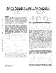
Minimum write access requirement without SE: This set of simulations does not consider SE and its BDD. Thus, the attacker can just focus on the sensors on the eight real tielines shown in Fig. 1. We evaluate the minimum number of tie-line sensors that the attacker needs to compromise in order to trigger remedial actions within two minutes. Fig. 14 shows this minimum number versus the setting of each element of amax , where amin = −amax . The decreasing trend suggests that, for a more stringent stealthiness constraint (i.e., a smaller amax ), the attacker needs to compromise more sensor data links to achieve a certain TTE. VIII. T ESTBED E XPERIMENTS We conduct experiments on a three-phase 16-bus 400 V power system testbed to evaluate the passive monitoring approach presented in Section V-B. The 16 buses, each installed in a cabinet as shown in Fig. 15(b), are connected to form a ring topology. Each bus is monitored by a smart meter. A variable load, as shown in Fig. 15(c), is connected to a bus in the system. Its power consumption can be tuned manually using a knob. A 13.5kVA generator, shown in Fig. 15(a), is driven by a motor (which simulates a turbine) and is connected to another bus in the system. The input power of the motor is supplied by a Current Vector Drive (CVD), which communicates with a remote computer. Power engineering researchers have implemented a single-area AGC algorithm using LabVIEW on the computer, which regulates the grid frequency based on a smart meter’s frequency measurements only. The LabVIEW program retrieves frequency measurements from the smart meter and sends the ACE to the CVD. Thus, different from the attacks on the power flow measurements described in the previous sections, in this section we study attacks on the frequency measurements and extend the passive monitoring approach to address this new attack model. Because of space constraints, the extension details are omitted here and can be found in [24]. The extended approach assumes that the attacker knows D, M , β, and can eavesdrop on the measurements of load deviation ∆p and frequency deviation ∆ω. We refer the reader to Section V-B for discussions on how the attacker can obtain these system constants and measurements. We conduct experiments to validate the extended passive monitoring approach. For this testbed, the constants needed by the attacker are D = −23 W/Hz, M = 2.6 kJ/Hz, and β = 300 W/Hz. The AGC cycle length is two seconds.

0.15 0.1 0.05 0 -0.05 -0.1 -0.15 50.2 50.1 50 49.9 49.8

a (Hz)

30

ground truth prediction

ω (Hz)

described in Eq. (4). Fig. 13 also shows the MTTE from a particular attack onset time versus |W|. The decreasing trend is consistent with the intuition that a less constrained attacker can cause a larger impact.

(c) variable load

Fig. 15. A 16-bus power system testbed.

Fig. 14. Minimum |W| yielding MTTE < 2 minutes.

MTTE (sec)

min |W|

8

820

830

840

850 860 Time (s)

870

880

Fig. 16. Top: injection to frequency readings. Bottom: frequency predicted by learned model and ground truth.

20 10 0 0.15

0.2 0.25 amax (Hz)

Fig. 17. MTTE vs. amax setting (amin = −amax ).

During the attacker’s learning phase, we manually tune the load to simulate load fluctuations. To mimic the attacker’s eavesdropping, we install Wireshark (a packet sniffer) on the computer running AGC and use it to extract ∆p and ∆ω from the network traffic. Using two minutes of eavesdropped data, we follow the extended passive monitoring approach [24] to learn the attack impact model using MATLAB’s system identification toolbox. We try different orders for some intermediate transfer functions to be identified and choose the orders that best fit the training data. The resulting transfer function for the FDI to the grid frequency is of the seventh order. We evaluate the learned attack impact model as follows. Using the model, we predict the trajectory of the grid frequency given a random attack sequence of limited magnitude, as shown in the top part of Fig. 16. Then, we inject this attack sequence to the real-time frequency measurements in the LabVIEW program during an experiment. We limit the magnitude of this test attack sequence to ensure that it will not cause damage to the testbed. The bottom part of Fig. 16 shows our prediction and the observed ground truth. The prediction matches the ground truth well and the mean absolute error of the prediction is 0.036 Hz only. This suggests that the learned model is accurate. With the learned model, we compute the optimal attack sequences under different settings for the FDI bound amax , where amin = −amax . Fig. 17 shows the computed MTTE versus amax . We can see that the MTTEs are below 30 seconds. Such short MTTEs suggest that it is critical to protect the frequency measurements of this testbed. Although we stop the experiment before physical damage happens on the testbed, the demonstrated accuracy of the learned attack impact model substantiates the importance of the optimal attacks in practice. IX. C ONCLUSION This paper studied FDI attacks on sensor data for AGC. We derived key attack impact models and showed that the attacker can learn the models based on eavesdropped sensor data and a modest amount of prior knowledge about the grid. Then, the attacker can compute an attack sequence to minimize

the remaining time before the grid must initiate costly and disruptive remedial actions such as disconnecting generators and customer loads. We developed an efficient algorithm to detect the attack and its onset time. Our analysis and algorithms were validated by experiments on a physical 16-bus power system testbed and extensive PowerWorld simulations based on a 37-bus power system model. ACKNOWLEDGEMENT This work was supported in part by the research grant for the Human-Centered Cyber-Physical Systems Programme at the Advanced Digital Sciences Center from Singapore’s Agency for Science, Technology and Research (A⋆STAR), and in part under the Energy Innovation Research Programme (EIRP, Award No. NRF2014EWTEIRP002-026), administrated by the Energy Market Authority (EMA). The EIRP is a competitive grant call initiative driven by the Energy Innovation Programme Office, and funded by the National Research Foundation (NRF). R EFERENCES [1] S. Karnouskos, “Stuxnet worm impact on industrial cyber-physical system security,” in 37th Conf. IEEE Ind. Electron. Society, 2011. [2] “Hackers infiltrated power grids,” 2014, http://on.recode.net/1FpKP7Y. [3] “The dragonfly attack,” 2014, http://rsa.dev.neptuneweb.com/ dragonfly-attack/. [4] Y. Liu, P. Ning, and M. K. Reiter, “False data injection attacks against state estimation in electric power grids,” in ACM CCS, 2009. [5] U.S. DHS, “Insider threat to utilities,” 2011, https://info. publicintelligence.net/DHS-InsiderThreat.pdf. [6] P. Kundur, N. J. Balu, and M. G. Lauby, Power system stability and control. McGraw-hill New York, 1994. [7] S. Sridhar and M. Govindarasu, “Model-based attack detection and mitigation for automatic generation control,” IEEE Trans. Smart Grid, vol. 5, no. 2, pp. 580–591, 2014. [8] S. Bhowmik, K. Tomsovic, and A. Bose, “Communication models for third party load frequency control,” IEEE Trans. Power Syst., vol. 19, no. 1, pp. 543–548, 2004. [9] K. Tomsovic, D. E. Bakken, V. Venkatasubramanian, and A. Bose, “Designing the next generation of real-time control, communication, and computations for large power systems,” Proc. IEEE, vol. 93, no. 5, pp. 965–979, 2005. [10] S. Sridhar and G. Manimaran, “Data integrity attacks and their impacts on scada control system,” in IEEE Power and Energy Society General Meeting, 2010. [11] “PowerWorld,” 2016, http://www.powerworld.com/. [12] “National grid maps,” 2016, http://www.geni.org/globalenergy/library/ national energy grid/. [13] Y. Chen, Z. Huang, Y. Liu, M. J. Rice, and S. Jin, “Computational challenges for power system operation,” in Hawaii International Conference on System Science, 2012. [14] S. Grijalva, “Research needs in multi-dimensional, multi-scale modeling and algorithms for next generation electricity grids,” 2011, http://1.usa. gov/1VBJAgu. [15] P. M. Esfahani, M. Vrakopoulou, K. Margellos, J. Lygeros, and G. Andersson, “Cyber attack in a two-area power system: Impact identification using reachability,” in ACC, 2010. [16] ——, “A robust policy for automatic generation control cyber attack in two area power network,” in IEEE CDC, 2010. [17] J. M. Hendrickx, K. H. Johansson, R. M. Jungers, H. Sandberg, and K. C. Sou, “Efficient computations of a security index for false data attacks in power networks,” IEEE Trans. Autom. Control, vol. 59, no. 12, pp. 3194–3208, 2014. [18] M. A. Rahman, E. Al-Shaer, and R. G. Kavasseri, “A formal model for verifying the impact of stealthy attacks on optimal power flow in power grids,” in ACM/IEEE ICCPS, 2014.

[19] S. Amin, X. Litrico, S. Sastry, and A. M. Bayen, “Cyber security of water scada systems–part i: analysis and experimentation of stealthy deception attacks,” IEEE Trans. Control Syst. Technol., vol. 21, no. 5, pp. 1963–1970, 2013. [20] A. A. C´ardenas, S. Amin, Z.-S. Lin, Y.-L. Huang, C.-Y. Huang, and S. Sastry, “Attacks against process control systems: risk assessment, detection, and response,” in ACM ASIACCS, 2011. [21] F. Pasqualetti, F. Dorfler, and F. Bullo, “Attack detection and identification in cyber-physical systems,” IEEE Trans. Autom. Control, vol. 58, no. 11, pp. 2715–2729, 2013. [22] H. Fawzi, P. Tabuada, and S. Diggavi, “Secure estimation and control for cyber-physical systems under adversarial attacks,” IEEE Trans. Autom. Control, vol. 59, no. 6, pp. 1454–1467, 2014. [23] A. Hahn, A. Ashok, S. Sridhar, and M. Govindarasu, “Cyber-physical security testbeds: Architecture, application, and evaluation for smart grid,” IEEE Trans. Smart Grid, vol. 4, no. 2, pp. 847–855, 2013. [24] Long version of this paper, Tech. Rep., 2016, http://publish.illinois.edu/ resilient-grid/files/2016/01/AGC-full.pdf. [25] “PJM manual 12,” 2015, http://www.pjm.com/markets-and-operations/ ancillary-services/∼ /media/documents/manuals/m12.ashx.

A PPENDIX : P ROOF

OF

P ROPOSITION 2

Proof. In Eq. (3), Φ−1 and Λ are the only unknowns. First, learn θ⊺ Φ−1 in Eq. (3) as a whole. Based on time series of ∆p and ∆ω computed from those of ∆pi and ∆ωi , apply system identification techniques (e.g., tfest in MATLAB) to fit θ ⊺ Φ−1 as a vector of N transfer functions. Try different orders for the transfer functions and choose orders that best fit the data. Second, as Λ appears in the coefficient of a only, we cannot learn Λ based on training data without a traces. We use its expression Λ = diag(sn1 − 1, . . . , snN − 1), where α K GY (s)T Y (s) ni = 1s + i i is2 i [24], and follow four steps: (i) Compute ∆pEi from ∆pij . With time series of ∆ωi , ∆pi , and ∆pEi , estimate the time series of (∆pYMi + ∆pN Mi ) based ^ ^ Y +∆p N −∆p gi −∆p ^ ∆p Ei Mi Mi g = ∆ωi described in Fig. 4(b). (ii) on Mi s+Di Estimate the time series of ACEi by ACEi = αi ∆pEi + N N ^ N = − Gi (s)Ti (s) ∆ω gi and βi ∆ωi . (iii) From Fig. 4(b), ∆p Mi RN i

Y Y Y Y ^ Y =− Gi (s)Ti (s) ∆ω gi − Gi (s)Ti (s)Ki · ACE ^i . The sum of ∆p Mi s RY i the two equations is a model with ∆ωi and ACEi as the inputs and (∆pYMi + ∆pN function for Mi ) as the output. The transfer GY (s)TiY (s)Ki ACEi in the summed model is Vi (s) = − i . With s time series of ∆ωi , ACEi , and (∆pYMi + ∆pN ), fit Vi (s). Mi (iv) Λ = diag(−α1 V1 (s), . . . , −αN VN (s)).

TABLE I S UMMARY OF N OTATIONS * Symbol ∆ωi ǫL ∆pEi αi , βi z W H a amin ∆pi ∆p ∆pij T Gi (s) K i , Ri Mi * Subscript

Definition Symbol grid freq. deviation ∆ω ∆ω lower bound ǫU power export deviation ACEi AGC algorithm constants m measurement vector N corruptible z element indices F regression horizon of Eq. (4) L FDI attack vector c lower bound for a amax change of load ℓij = [∆p1 , . . . , ∆pN ]⊺ uh , v h power flow deviation of ℓij Ψ, Λ, Φ (Tz)[i] is a tie-line flow ∆pM i speed controller transfer func. Ti (s) generator constants Di total generator inertia θ i refers to area i. “Tie-line” refers to virtual

Definition avg grid freq. deviation ∆ω upper bound area control error number of sensors number of areas measurement matrix of SE number of tie-lines injected SE error upper bound for a tie-line from area i to j coefficients in Eq.(4) parameters of Eq. (3) mechanical power change turbine transfer function load-damping constant 1 = N · [1, 1, . . . , 1]⊺ tie-line.