Optimal Finite-Horizon Sensor Selection for Boolean Kalman Filter Mahdi Imani and Ulisses M. Braga-Neto Department of Electrical and Computer Engineering Texas A&M University College Station, TX USA Email:
[email protected],
[email protected]
Abstract—Partially-observed Boolean dynamical systems (POBDS) are large and complex dynamical systems capable of being monitored through various sensors. However, limitations such as time-limit constraints, the availability of physical or storage space, and economical constraints impede the use of all sensors for estimation purposes. Thus, developing a procedure for selecting a subset of the sensors is essential. The optimal minimum mean-square error (MMSE) POBDS state estimator is the Boolean Kalman Filter (BKF) and Smoother (BKS). Naturally, the performance of these estimators strongly depends on the choice of sensors. Given a finite subsets of sensors, for a POBDS with a finite observation space, we introduce the optimal procedure to select the best subset which leads to the smallest expected mean-square error (MSE) of the BKF over a finite horizon. The performance of the proposed sensor selection methodology is demonstrated by numerical experiments with a p53-MDM2 negative-feedback loop gene regulatory network observed through Bernoulli noise. Index Terms—Optimal Finite-Horizon Sensor Selection, Partially-Observed Boolean Dynamical Systems, Boolean Kalman Filter, Gene Regulatory Networks.
Therefore, selecting the appropriate subset of sensors before starting the estimation process is crucial. Sensor selection is widely discussed in the literature for both linear [17]–[19] and nonlinear dynamical systems [16], [20]–[23]. These methods use various objective functions such as the Chernoff and Kullback-Leibler distances [26], information gain [27], and estimation error [28]. However, due to the derivativeless nature of the Boolean state equation in a POBDS, none of the mentioned sensor selection methods are directly applicable here. This paper introduces an optimal methodology for selecting the best sensor to minimize the expected mean-square error (MSE) of a BKF with finite measurement space over a finitehorizon. Performance is investigated using a Boolean network model of the p53-MDM2 negative feedback loop network observed through Bernoulli noise.
I. I NTRODUCTION
We assume that the system is described by a state process {Xr ; r = 0, 1, . . . , T }, for a finite horizon T , where Xr ∈ {0, 1}d is a Boolean vector of size d. The states are assumed to be updated at each discrete time through the following Boolean signal model:
Partially-observed Boolean dynamical systems (POBDS) [1], [2] offer a rich framework for estimation and prediction in fields as varied as genomics [3], robotics [4], and digital communications [5], and more. The optimal recursive minimum mean-square error (MMSE) POBDS state estimators are the Boolean Kalman Filter (BKF) [2] and Smoother (BKS) [6]. Several other tools have been developed for the POBDS model in recent years, such as particle filters for state and parameter estimation [7], schemes for simultaneous state and parameter estimation [1], optimal filter with correlated observation noise [8], network inference [9], and control [10]–[13]. Most of these tools are freely available through an open-source R package called “BoolFilter” [14], [15]. POBDSs can be monitored through various sensors that carry information about different parts of the system with various degrees of uncertainty. However, the number of sensors is often limited either by economical constraints (hardware costs), or the availability of physical or storage space [16]. While the BKF is the optimal MMSE POBDS state estimator, its performance strongly depends on the choice of sensors.
II. PARTIALLY-O BSERVED B OOLEAN DYNAMICAL S YSTEMS
Xr = f (Xr−1 , ur ) ⊕ nr ,
(1)
for r = 1, . . . , T . Here, ur ∈ {0, 1}d is an input at time r which is assumed to be deterministic and known, nr ∈ {0, 1}d is Boolean transition noise at time r, “⊕” indicates componentwise modulo-2 addition, and f is the network function. The states are observed indirectly through the observation process {Yr ; r = 1, . . . , T }. In this paper, we assume a simple additive-noise Boolean observation model: Yr = Xr ⊕ v r ,
(2)
for r = 1, . . . , T , where vr ∈ {0, 1}d is Boolean observation noise at time r. Hence, Yr ∈ {0, 1}d is a Boolean observation vector at time r. Both noise processes {nr ; r = 1, . . . , T } and {vr ; r = 1, . . . , T } are assumed to be “white” in the sense that the noises at distinct time points are independent. It is also assumed that the noise processes are independent from
each other and from the initial state X0 ; their distribution is otherwise arbitrary. The optimal filtering problem consists of, given observations ˆ MS of Y1∶r = (Y1 , . . . , Yr ), for r ≤ T , finding an estimator X r∣r the state Xr that minimizes the conditional mean-square error (MSE): ˆ r∣r ∣ Y1∶r ) = E [∣∣X ˆ r∣r − Xr ∣∣2 ∣ Y1∶r ] , MSE(X
(3)
where ∣∣v∣∣ = is the square of the L2 norm of vector v. Clearly, for Boolean vectors, ∣∣v∣∣2 = ∣∣v∣∣1 = ∑di=1 ∣v(i)∣ is the L1 norm of v. ˆ MS , We present next a recursive algorithm to compute X r∣r known as the Boolean Kalman Filter (BKF) [?], [2]. Define the conditional probability distribution vectors: 2
Algorithm 1 Boolean Kalman Filter 1:
Initialization: (Π0∣0 )i = P (X0 = xi ) , for i = 1, . . . , 2d . For r = 1, . . . , T , do:
2:
Prediction: Πr∣r−1 = Mr Πk−1∣k−1
3:
Update: β r = Tr (Yr ) Πr∣r−1
4:
Filtered Distribution Vector: Πr∣r = β r /∣∣β r ∣∣1
d ∑i=1 v(i)2
Πr∣r (i) = P (Xr = xi ∣ Y1∶r ) , Πr∣r−1 (i) = P (Xr = xi ∣ Y1∶r−1 ) ,
= P (nr = f (xj , ur ) ⊕ xi ) ,
ˆ MS = AΠr∣r X r∣r 6:
Optimal Conditional MSE:
(4)
(5)
for i, j = 1, . . . , 2d . Additionally, given a value of the observation vector Yr at time r, the update matrix Tr (Yr ) of size 2d × 2d is a diagonal matrix defined by: (Tr (Yr ))ii = P (Yr ∣ Xr = xi ) ,
MMSE Estimator Computation:
ˆ MS ∣ Y1∶r ) = ∣∣ min{AΠr∣r , (AΠr∣r )c }∣∣1 MSE(X r∣r
for i = 1, . . . , 2d , and r = 1, . . .. Notice that Π0∣0 is the initial (prior) distribution of the states at time zero. Let Mr be the transition matrix of the Markov chain defined by the state model, specified by: (Mr )ij = P (Xr = xi ∣ Xr−1 = xj )
5:
(6)
for i = 1, . . . , 2d . d Finally, let A = [x1 ⋯x2 ] be a d×2d matrix with all possible state vectors as columns. In addition, for a vector v of size d, define v ∈ {0, 1}d via v(i) = Iv(i)>1/2 for i = 1, . . . , d, and vc ∈ {0, 1}d via vc (i) = 1 − v(i), for i = 1, . . . , d; where Iv(i)>1/2 returns 1 if v(i) > 1/2 and 0 otherwise. The full procedure of the BKF is presented in Algorithm 1.
entire interval r = 1, . . . , T while achieving the best possible performance, as defined below. The problem of scheduling different sensors at different times will be considered in future work. m Let Om r be the space of observation sequences Y1∶r provided by the mth sensor up to time r. Note that in the setting m assumed in this paper, Orm is finite, with ∣Orm ∣ = 2∣Y ∣×r . Let m Xr∣r be the set of all estimators of Xr based on observations m Y1∶r ∈ Orm , for m = 1, . . . , M . Before execution, we do not m know the specific realization Y1∶r for any of the sensors. Therefore, we consider the expected MSE and define the optimal estimator: ˆ r∣r ∣ Ym )]. ˆ m,MS = argmin E[MSE(X X 1∶r r∣r
We then select the sensor that achieves the best average expected MSE over the interval r = 1, . . . , T : m∗ = argmin m=1,...,M
III. F INITE -H ORIZON S ENSOR S ELECTION Suppose that one would like to select among M available sensors, where each sensor is a fixed vector function of the observation vector Yr . In this paper, we consider a simple case where each sensor corresponds to a different subset of the measurements in Yr , but linear and nonlinear combinations of all or a subset of the measurements may be considered as well. m Hence, we have M sensors Ym = {ym,1 , . . . , ym,∣Y ∣ }, for m = 1, . . . , M , which are different subsets of the available observation vector Y. The value obtained by the mth sensor at time r is: m Yrm = Xm (7) r ⊕ vr , m where Xm r and vr are the corresponding subsets of the state Xr and observation noise vr at time r. The goal is to select a sensor, before the start of the filtering process, to use over the
(8)
ˆ m ∈X m X r∣r r∣r
1 T ˆ m,MS ∣ Ym )] . ∑ E[MSE(X 1∶r r∣r T r=1
(9)
From Algorithm 1, we have that: ˆ m,MS ∣ Ym )] E[MSE(X 1∶r r∣r m c = E[∣∣ min{AΠm r∣r , (AΠr∣r ) }∣∣1 ]
=
(10)
m m m c ∑ P (Y1∶r ) ∣∣ min{AΠr∣r , (AΠr∣r ) }∣∣1 .
m ∈O m Y1∶r r
ˆ m,MS ∣ Ym )] exactly thus requires, in Calculating E[MSE(X 1∶r r∣r principle, the computation of the conditional MSE given all possible sequences of measurements. Since the observation space Orm is finite, this computation is possible, as described next, provided that the sensor dimensionalities ∣Ym ∣ and horizon T are small enough. Approximations for the case of large sensor dimensionalities and long horizons will be dealt with in future work.
Given that Π0∣0 is the initial distribution vector, the posterior distribution at time 1 associated to measurement ym,j can be computed using the Bayes’ rule as: Πm,j = P (X1 ∣ Y1m = ym,j ) = 1∣1
T1 (ym,j ) M1 Π0∣0 , (11) ∣∣T1 (ym,j ) M1 Π0∣0 ∣∣1
for j = 1, ..., 2∣Y ∣ . (Notice that there is no superscript “m” over X1 .) The probability of observing ym,j at time step 1 can be computed as follows: m
w1m,j = P (Y1 = ym,j ∣ Π0∣0 ) = ∣∣T1 (ym,j ) M1 Π0∣0 ∣∣1 , (12) m for j = 1, ..., 2∣Y ∣ . This process can be continued recursively to compute all needed probabilities, as illustrated in Figure 1.
noisy measurements. We base our experiments on the wellknown p53-MDM2 negative-feedback gene regulatory network [?]. The pathway diagram for this network is presented in Fig. 2. The p53 gene codes for the tumor suppressor protein p53 in humans, and its activation plays a critical role in cellular responses to various stress signals that might cause genome instability. The gene regulatory network consists of four genes: ATM, p53, Wip1, and MDM2, and the input “dna dsb”, which indicates the presence of DNA double strand breaks. The Boolean function is represented by the following logic functions: ATMk = WIP1k−1 AND dna dsb p53k = ATMk−1 AND WIP1k−1 AND MDM2k−1 WIP1k = p53k−1 MDM2k = (ATMk−1 AND (p53k−1 OR WIP1k−1 )) OR (p53k−1 AND WIP1k−1 )
DNA DSBs
…
ATM
…
Fig. 1: Posterior distribution tree for mth sensor. The entire process of finite-horizon sensor selection for the BKF is presented in Algorithm 2. Algorithm 2 Optimal Finite-Horizon Sensor Selection for the BKF 1: Posterior Distributions Computation: For m ∈ {1, ..., M }, do: − Initialization: Πm,1 = Π0∣0 , w0m,1 = 1. 0∣0 For r = 1, ..., k, do: For i = 1, ..., 2∣Y −
Πm,i r∣r−1
=
m
∣(r−1)
, do:
Mr Πm,i . r−1∣r−1
For j = 1, ..., 2∣Y ∣ , do: m
m,(i−1)2∣Y
− Πr∣r
m,(i−1)2∣Y
− wr 2:
m∣
m∣
+j
+j
=
Tr (ym,j ) Πm,i r∣r−1 ∣∣Tr (ym,j ) Πm,i ∣∣ r∣r−1 1
.
m,i = {wr−1 ∣∣Tr (ym,j ) Πm,i ∣∣ }. r∣r−1 1
The Optimal Selected Sensor: ∗
k 2∣Y
m ∣r
m = argmin ∑ ∑ wrm,i ∣∣ min{AΠm,i , (AΠm,i )c }∣∣1 r∣r r∣r m∈{1,...,M } r=1
p53
…
…
…
…
…
i=1
IV. N UMERICAL E XPERIMENTS In this section, we describe an application of our methodology to Boolean gene regulatory networks observed through
WIP1
MDM2
Fig. 2: Activation/repression pathway diagram of the P53MDM2 negative feedback loop Boolean network. The process noise is assumed to have independent components distributed as Bernoulli, with intensity p, so that all genes are perturbed with a small probability. We assume the states are observed through i.i.d. Bernoulli noise with parameter q the same for all genes. Four sensors are assumed in this numerical experiment (M = 4), in which each sensor consists of the noisy observation of one of the genes in the network. The average expected optimal MSE of the BKF over a time horizon 10 for various sensors are presented in Table I. The average expected optimal MSE is larger for larger observation noise. Furthermore, one can also see that the average expected error is larger in the case of an active dna dsb input in comparison to an inactive one. This can be explained by the attractor structure of the p53-MDM2 Boolean network in the presence and absence of external input, in which the system has a singleton and cyclic attractor in the absence and presence of DNA damage, respectively. For more information, see [?]. The optimal sensor is specified by bold numbers in Table 1. One can see that in the case of an inactive dna dsb input, MDM2 is the best choice in all cases. With an active dna dsb input, either ATM, p53 or Wip1 sensors are the best choices, depending on the parameters of the system. For example, the choices of optimal sensor in the case of small process and observation noise are different for two initial distribution
TABLE I: Optimal Finite-Horizon Sensor Selection Results for Horizon T = 10. No stress (dna dsb = 0) q
p
0.01 0.05
ATM
p53
Wip1
Mdm2
ATM
p53
Wip1
Mdm2
1 1 T [ 16 , ..., 16 ]
0.2750741
0.2638027
0.1656234
0.1068837
1.474933
1.495893
1.443079
1.733152
[0, ..., 1]T
0.3759515
0.3700666
0.336286
0.2862778
1.557895
1.564755
1.569989
1.709767
0.7762779
0.7450073
0.5673365
0.4586170
1.218192
1.371414
1.25308
1.480116
[0, ..., 1]T
0.8456097
0.8206338
0.6542587
0.5223727
1.261300
1.395272
1.284143
1.431346
1 1 T [ 16 , ..., 16 ]
0.2763222
0.2666612
0.187685
0.1429032
1.582349
1.546739
1.520243
1.767097
[0, ..., 1]T
0.3771996
0.3721163
0.3515226
0.3258301
1.682476
1.650215
1.658933
1.753322
0.7896947
0.7643199
0.6193023
0.5399353
1.351779
1.420585
1.342386
1.528136
0.8590265
0.8387905
0.7193224
0.6283275
1.388158
1.443909
1.383008
1.509838
1 , ..., [ 16
0.1
0.01 0.15
1 , ..., [ 16
0.1
DNA damage (dna dsb = 1)
Initial Distribution
1 T ] 16
1 T ] 16
[0, ..., 1]T
vectors. The similar trend can be seen in the case of large measurement noise. From the results of Table I, one can clearly understand the importance of the sensor selection process, and its dependency on the initial distribution, the values of noise and input to the system. The effect of the length of horizon on the choice of optimal sensor is investigated next. The parameters used are Π0∣0 = [0, ..., 1]T , p = 0.01, q = 0.05 and dna dsb = 1. The average expected MSE over time-horizon of the optimal filter for different choices of sensors and various time-horizons is presented in Fig. 3. As it is clear in Fig. 3, for time-horizons 1, 6-8, 11-13 and 15, observing the Wip1 gene will result in the minimum expected MSE of the BKF, for time steps 2 and 3, Mdm2 has the lowest expected optimal MSE, and for the intervals 4-5, 9-10 and 14 the best sensor is ATM. This emphasizes the difficulty and importance of the sensor selection procedure.
Average Expected MSE
ATM p53 Wip1 Mdm2
Time-Horizon
Fig. 3: Average expected optimal MSE for different choices of sensors and time-horizons.
V. C ONCLUSION We developed an optimal finite-horizon sensor selection procedure for state estimation for POBDS models with a finite observation space. The sensor selected by the developed method is guaranteed to yield the minimum expected meansquare error (MSE) for the optimal filter. Performance was investigated using a model of the p53-MDM2 negative feedback loop network. Future work will include the use of more complex sensor models and approximations for large sensor dimensionality and long time horizons. ACKNOWLEDGMENT The authors acknowledge the support of the National Science Foundation, through NSF award CCF-1320884. R EFERENCES [1] M. Imani and U. Braga-Neto, “Maximum-likelihood adaptive filter for partially-observed Boolean dynamical systems,” IEEE Transactions on Signal Processing, vol. 65, no. 2, pp. 359–371, 2017. [2] U. Braga-Neto, “Optimal state estimation for Boolean dynamical systems,” in Signals, Systems and Computers (ASILOMAR), 2011 Conference Record of the Forty Fifth Asilomar Conference on, pp. 1050–1054, IEEE, 2011. [3] S. Kauffman, “Metabolic stability and epigenesis in randomly constructed genetic nets,” Journal of Theoretical Biology, vol. 22, pp. 437– 467, 1969. [4] A. Roli, M. Manfroni, C. Pinciroli, and M. Birattari, “On the design of Boolean network robots,” in Applications of Evolutionary Computation, pp. 43–52, Springer, 2011. [5] D. Messerschmitt, “Synchronization in digital system design,” IEEE Journal on Selected Areasin Communications, vol. 8, no. 8, pp. 1404– 1419, 1990. [6] M. Imani and U. Braga-Neto, “Optimal state estimation for Boolean dynamical systems using a Boolean Kalman smoother,” in Proceedings of the 3rd IEEE Global Conference on Signal and Information Processing (GlobalSIP’2015), Orlando, FL, pp. 972–976, IEEE, 2015. [7] M. Imani and U. Braga-Neto, “Particle filters for partially-observed Boolean dynamical systems,” Automatica, 2017. [8] L. McClenny, M. Imani, and U. Braga-Neto, “Boolean Kalman filter with correlated observation noise,” in Proceedings of the 42nd IEEE International Conference on Acoustics, Speech and Signal Processing (ICASSP 2017), New Orleans, LA, IEEE, 2017. [9] M. Imani and U. Braga-Neto, “Optimal gene regulatory network inference using the Boolean Kalman filter and multiple model adaptive estimation,” in Proceedings of the 49th Annual Asilomar Conference on Signals, Systems, and Computers, Pacific Grove, CA, pp. 423–427, IEEE, 2015.
[10] M. Imani and U. Braga-Neto, “Control of gene regulatory networks with noisy measurements and uncertain inputs,” IEEE Transactions on Control of Network Systems, 2018. [11] M. Imani and U. Braga-Neto, “Multiple model adaptive controller for partially-observed Boolean dynamical systems,” in Proceedings of the 2017 American Control Conference (ACC2017), Seattle, WA, 2017. [12] M. Imani and U. Braga-Neto, “Point-based value iteration for partiallyobserved Boolean dynamical systems with finite observation space,” in Decision and Control (CDC), 2016 IEEE 55th Conference on, pp. 4208– 4213, IEEE, 2016. [13] M. Imani and U. Braga-Neto, “State-feedback control of partiallyobserved Boolean dynamical systems using RNA-seq time series data,” in American Control Conference (ACC), 2016, pp. 227–232, IEEE, 2016. [14] L. D. McClenny, M. Imani, and U. M. Braga-Neto, “BoolFilter: an R package for estimation and identification of partially-observed Boolean dynamical systems,” BMC bioinformatics, 2017. [15] L. D. McClenny, M. Imani, and U. Braga-Neto, “BoolFilter package vignette,” The Comprehensive R Archive Network (CRAN), 2017. [16] S. P. Chepuri and G. Leus, “Sparsity-promoting sensor selection for nonlinear measurement models,” IEEE Transactions on Signal Processing, vol. 63, no. 3, pp. 684–698, 2015. [17] R. Mehra, “Optimization of measurement schedules and sensor designs for linear dynamic systems,” IEEE Transactions on Automatic Control, vol. 21, no. 1, pp. 55–64, 1976. [18] V. Gupta, T. H. Chung, B. Hassibi, and R. M. Murray, “On a stochastic sensor selection algorithm with applications in sensor scheduling and sensor coverage,” Automatica, vol. 42, no. 2, pp. 251–260, 2006. [19] S. Liu, M. Fardad, E. Masazade, and P. K. Varshney, “Optimal periodic sensor scheduling in networks of dynamical systems,” IEEE Transactions on Signal Processing, vol. 62, no. 12, pp. 3055–3068, 2014. [20] A. Doucet, B.-N. Vo, C. Andrieu, and M. Davy, “Particle filtering for multi-target tracking and sensor management,” in Information Fusion, 2002. Proceedings of the Fifth International Conference on, vol. 1, pp. 474–481, IEEE, 2002. [21] B.-N. Vo, S. Singh, and A. Doucet, “Sequential Monte Carlo methods for multitarget filtering with random finite sets,” IEEE Transactions on Aerospace and electronic systems, vol. 41, no. 4, pp. 1224–1245, 2005. [22] A. Sarrafi and Z. Mao, “Probabilistic uncertainty quantification of wavelet-transform-based structural health monitoring features,” in SPIE Smart Structures and Materials+ Nondestructive Evaluation and Health Monitoring, pp. 98051N–98051N, International Society for Optics and Photonics, 2016. [23] A. Sarrafi and Z. Mao, “Uncertainty quantification of phase-based motion estimation on noisy sequence of images,” in SPIE Smart Structures and Materials+ Nondestructive Evaluation and Health Monitoring, pp. 101702M–101702M, International Society for Optics and Photonics, 2017. [24] S. Ghoreishi and D. Allaire, “Adaptive uncertainty propagation for coupled multidisciplinary systems,” AIAA Journal, 2017. [25] S. F. Ghoreishi and D. L. Allaire, “Compositional uncertainty analysis via importance weighted gibbs sampling for coupled multidisciplinary systems,” in 18th AIAA Non-Deterministic Approaches Conference, p. 1443, 2016. [26] D. Bajovic, B. Sinopoli, and J. Xavier, “Sensor selection for event detection in wireless sensor networks,” IEEE Transactions on Signal Processing, vol. 59, no. 10, pp. 4938–4953, 2011. [27] F. Zhao, J. Shin, and J. Reich, “Information-driven dynamic sensor collaboration,” IEEE Signal processing magazine, vol. 19, no. 2, pp. 61– 72, 2002. [28] S. Joshi and S. Boyd, “Sensor selection via convex optimization,” IEEE Transactions on Signal Processing, vol. 57, no. 2, pp. 451–462, 2009.