Optimal Integrated Call Admission Control and ... - Semantic Scholar

Optimal Integrated Call Admission Control and Dynamic Pricing with Handoffs and Price-Affected Arrivals Siew-Lee Hew and Langford B. White Centre for Internet Research (CIR), The University of Adelaide, SA 5005, Australia. Email: [email protected], [email protected]

Abstract— Call admission control and dynamic pricing have been proposed as separate measures to reduce congestion in a network. In this paper, we integrate the call admission control and dynamic pricing problems, formulating them as a Markov Decision Problem (MDP), operating in a multiservice, resourcesharing cellular system. Our model incorporates price-affected behaviour of network users, considering effects on arrivals, retrials and substitutions among services and time. The network exercises admission control, to reject or accept a new connection requests, and price control to set a state-dependent price per bandwidth time with the objective to maximise the long-term revenue. The results show that the proposed method improves revenue and reduces congestion compared to other conventional sub-optimal policies.

New Arrivals λ 0j

Deferred Arrivals xj σj

upj

Price Control

Orbit j Insufficient WTPj

λ

Blocked Call Admission Control

Retry αRj

αSOjk αAj

αSOkj

Substitute In Substitute Out Abandon

ucj

Admitted Users

Fig. 1.

Integrated Call Admission and Dynamic Pricing Model.

I. I NTRODUCTION Call admission control (CAC) and dynamic pricing have been proposed as arbitration mechanisms to regulate traffic and reduce congestion in a network. CAC is such a provisioning strategy to limit the number of call connections. It means that users are not automatically admitted even though there are resources available. Dynamic pricing makes adjustments often, according to the demand pattern and congestion level in a network in order to influence the way users utilise network resources, especially to allocate limited resources to those who value them most. Dynamic pricing also enhances network operators’ ability to recover costs and make profits to finance capacity expansions. By influencing the demand patterns, operators could avoid the costly need to provision a network so that it can always meet its peak demand. Many pricing schemes have been put forward. The concept of auction-based, smart-market pricing is proposed in [1]. A charge that is based on effective bandwidth is constructed in [2].Charges depend upon both static parameters, being traffic contracts, and dynamic measures, being the current usage of network resources. Pricing models in multiservice networks have been considered in [3] for the single link case and in [4] for the network case, where near-optimal static pricing policies have been established for a network with many small sources of traffic. We refer our readers to [5] for a comprehensive survey on the vast number of pricing schemes proposed. These schemes are proposed for broadband networks like the Internet where resource reservation for handoff users is a non-issue. In this paper, we provide a generic framework to formulate an integrated call admission and dynamic pricing problem for multiservice, resource-sharing cellular systems as a Markov Decision Problem (MDP) and solve it using dynamic programming methods [6]. The objective is to maximise the long-term

expected revenue. Given a particular configuration of network users, the objective is to determine both whether or not to accept a new connection and the optimal price per bandwidth time to shape demand. Since premature termination of ongoing calls is more undesirable than rejection of new call requests, it has been widely accepted that a system should allocate a higher priority to handoff call requests. Our model allows for bandwidth reservation for handoff calls by associating a Satisfaction Revenue (SR) with the admission of handoff calls. SR is not a real income to the service operator. A major and inaccurate assumption in all of the papers mentioned is that users arrive independently according to a Poisson process and will be automatically lost if blocked. This queueing model creates an underestimation of the actual arrival rate in the system, especially during congestion. As depicted in Fig. 1, we consider an advanced arrival model that incorporates retrials and substitution effects among services and through time. Assuming that some users remain in the vicinity of the system when blocked, they have a choice to defer their call requests or to use another service as a substitute. These deferred users, together with new arrivals, provide a more realistic estimate of the actual arrival rate to the system than do conventional arrival models. However, handoff connection requests are not price-affected since they are pre-admitted at other prices and are assumed to leave the system if blocked. A similar work has been considered in [7]. In their work, the dynamic pricing component of the integrated system is only active when the arrival rate of the system exceeds a pre-determined optimal level. Instead, we will use prices as incentive to encourage arrivals during low-traffic period, in addition of congestion control during high-traffic period. The CAC component of [7] only assumes a certain number of guard

channels and, unlike our work, does not optimally reserve resources for future-arriving handoff and new users that will maximise the long-term revenue. Besides, our problem is different because we consider the integrated problem in a decision-theoretic framework and solve it using different tools. The rest of the paper is organised as follows. In Section II, we describe our network model. We then formulate our integrated problem in section III and present computational results in Section IV. Conclusions are summarised in Section V. II. N ETWORK M ODEL We consider a network with B units of bandwidth and J classes of service. The price per unit time for using one unit of bandwidth of service class j is denoted as upj , j = 1, 2, . . . , J. Each service class j, which uses bj units of bandwidth, is characterised by its Poisson-distributed new and handoff call arrival rates λnj and λhj , exponentially-distributed call holding time 1/µj and Weibull-distributed willingness to pay (WTP) Ψj with mean ψj and shape βj . WTP quantifies the satisfaction gained from a call. We use the Weibull distribution to model users’ WTP because it is versatile and can take up the characteristics of other types of distributions, based on the value of the shape parameter. Within the telecommunications framework, it has been used to model the traffic characteristics of packet audio streams in [8] and to simulate data traffic in [9]. Different values of the shape parameter have different effects on the behaviour of the distribution. Exponential demand functions (β = 1), as used in [7], are special instances of the WTP distribution considered in this work. CAC is triggered when a user makes a call connection request. At the time a new or handoff call is accepted, the system must have at least bj units of bandwidth available. A handoff connection request will always be accepted if the system has sufficient bandwidth. A CAC policy determines the statedependent admission policy, uc (s) = (uc1 (s), . . . , ucJ (s)), for new users, for every state s. A new connection can either be accepted with ucj = 1 or rejected with ucj = 0. A new user will decide to either make a connection request if his or her budget is sufficient to cover the expected call cost, i.e. Ψj ≥ upj bj /µj or defer the request otherwise. When blocked, handoff users will leave the system immediately. However, new users of service j who are rejected by control or have insufficient WTP will either retry later with probability αRj , substitute out to another service k 6= j, with probability αSOjk or abandon the system with probability αAj . New users of service j who retry later and users of service k 6= j who substitute in to service j are said to be in orbit and will independently generate requests for service at exponentially-distributed time intervals with mean 1/σj until they obtain service, abandon or substitute out. Price control determines the state-dependent pricing vector up (s) = (up1 (s), . . . , upJ (s)), with upj ∈ Upj , to regulate new call arrivals to the network. Upj is the set of possible values of upj . Therefore, the demand for service of new users depends on upj , the desired service length and their WTP. We

denote the probability of having the sufficient WTP to make a call as the access probability: αPj = 1 − FW (upj bj /µj ),

(1)

where FW (y) = P [Ψj ≤ y | ψj , βj ] is the cumulative distribution function of the Weibull-distributed Ψj . λnj is the maximum new arrival rate, limited by the access probability αPj . The total price-affected arrival rate to a service is therefore λj = αPj (λnj +xj σj ), where xj is the number of users in orbit and σj is the retrial rate of these users. Access probability can be seen as an arrival gate that controls the flow of priceaffected arrivals to the system. By varying upj , the arrival rate of a particular service can be encouraged or discouraged to give way for arriving handoff or higher revenue-generating users. The objective is to exercise call admission and pricing to maximise the long-term expected revenue. As mentioned in [7], the parameters that define the WTP distribution function must be identified by adequate market research. In reality, the information on users’ call budget can be extracted from an operator’s historical data on users’ spending patterns and expenditure. Users can also willingly inform network operator of their WTP and this procedure can be automated by including a simple call-budgeting program in users’ mobile device. Although it is expected that most users would like to spend as little as possible and only indicate their minimum WTP, higher-end users would place a higher value on a call during congestion when their initial WTP is not sufficient. III. M ARKOV D ECISION P ROBLEM F ORMULATION The system can be described by a Markov Chain on the state space S = {(x, n) : 0 ≤ xj ≤ Xj , n0 b ≤ B, ∀j ≤ J}. Vectors n = (n1 , . . . , nJ ), x = (x1 , . . . , xJ ) and b = (b1 , . . . , bJ ) denote the number of active connections, the number of users in orbit and the amount of bandwidth required for all services respectively. To ensure that the state space remains finite, we limit the number of users in orbit to X. When the number of users in the orbit of service j reaches Xj , the blocked calls will be lost and no users from other services can substitute in. This truncation method is often used in the analysis of retrial system to reduce the complexity involved and methods of choosing appropriate level of truncation are discussed in [10]. We will now derive the transition rates from a state s = (x, n). The number of active connections in the system increases due to arriving handoff users at a rate of: q((x, n), (x, n + ej )) = λhj I(n0 b + bj ≤ B) = λ0j .

(2)

The value of an indicator function I(a) is 1 if condition a is true and 0 otherwise. New and retrying users in orbit increase the number of connections at the following rates respectively q((x, n), (x, n + ej )) q((x, n), (x − ej , n + ej ))

= αPj λnj ucj = λ1j

(3)

= αPj xj σj ucj = λ2j (4)

where ej is a unit vector with 1 in its j th position. The number of connections will decrease at a rate of: q((x, n), (x, n − ej )) = nj µj I(nj > 0).

(5)

The number of users in orbit j will only decrease if users abandon service at a rate of q((x, n), (x − ej , n)) = (1 − αPj ucj )αAj xj σj = λ3j

(6)

or substitute out to another service k, k 6= j, at q((x, n), (x − ej + ek , n)) = (1 − αPj ucj )αSOjk xj σj = λ4jk . (7) The number of users in orbit j will increase if new users retry at a rate of q((x, n), (x + ej , n)) = (1 − αPj ucj )αRj λnj + J X

(8)

(1 − αPk uck )αSOkj λok = λ5j

k6=j

or users of another service, say k where k 6= j, substitute in at a rate of q((x, n), (x+ej −ek , n)) = (1−αPk uck )αSOkj xk σk = λ4kj . (9) Note that (7) and (9) are actually the same. In order to avoid calculating the same rates twice, we only need to consider the rates associated with a user substituting out for each service. We also note that transitions q((x, n), (x − ek , n + ej )) are disallowed and set to zero. This means that users substituting in from service k need to enter the orbit of service j before reattempting. Users who reattempt unsuccessfully and decide to reattempt again, and new users who abandon do not change the state of the system. Even though the process evolves in continuous time, we only have to consider the state of the network when certain events take place. We say that an event happens at a certain time if any of the transitions derived in the previous section occurs. Let Ω denote the set of possible events, i.e. Ω = {ω | ω ∈ {0, 1, 2, 3, 4, 5, 6, 7}J }. The list of possible events corresponds to the possible transitions outlined previously, i.e. event 0 indicates an handoff arrival, 1 indicates a new arrival, 2 indicates an arrival from orbit and so on. Event 7 indicates no event occurring. For each state s ∈ S and event ω ∈ Ω, U (s, ω) is the set of available decisions: ( {Uc × Up } if ω ∈ Ωa (10) U (s, ω) = {Up } if ω ∈ / Ωa , where Ωa is the set of all events consisting of arrival events 1 or 2. Uc and Up denote the set of all possible call admission and price control decisions and are defined as Uc = {uc | ucj ∈ {0, 1}, ∀j} and Up = {up | upj ∈ Upj , ∀j} respectively. Given that the system is in state s ∈ S with control actions u ∈ U available and an event ω ∈ Ω occurred, the next state,

s0 ∈ S, is given by a function f : S × Ω × U such that   (x, n + ej ) if ωj = 0, n0 b + bj ≤ B     if ωj = 1, ucj = 1  (x, n + ej )    (x − ej , n + ej ) if ωj = 2, ucj = 1    (x − e , n) if ωj = 3 j f (s, ω, u) = (11)  (x − ej + ek , n) if ωj = 4      (x + ej , n) if ωj = 5     (x, n − ej ) if ωj = 6     (x, n) otherwise. Using uniformisation [6], the continuous-time MDP can be transformed into its discrete-time equivalence with the socalled uniform transition rate, where the total transition rate out of any state is bounded by ν. The transition probabilities p(s, ω, u) for state s are then given by λ 0j  if ωj = 0  ν   λ 1j  if ωj = 1   ν    λ2j if ωj = 2  ν    λ3j if ωj = 3 (12) p(s, ω, u) = λν4jk  if ωj = 4  ν   λ5j   if ωj = 5  ν   nj µj  if ωj = 6  ν    and if ωj = 7, 1 − ν(s) ν

where the PJtotal transition rate out of state s ∈ S is given by ν(s) = j=1,k6=j λ0j + λ1j + λ2j + λ3j + λ4jk + λ5j + nj µj . The revenue rate collected by the system at a particular state s = (x, n) is be given by the reward function   if ωj = 0 and n0 b + bj ≤ B SR g(s, ω, u) = rj = upj bj /µj if ωj = 1, 2 and ucj = 1   0 otherwise. (13) Reward rj is the revenue collected when a user of class j is admitted. In order to reflect the higher importance of accepting handoff calls, SR should be greater than the actual revenue provided by the admission of new call requests. A user is admitted based on a single admission price that will not change for the entire duration of the call. The average reward-to-go function is given by the Bellman’s equation: " # X ∗ 0 J + h(s) = max p(s, ω, u)[g(s, ω, u) + h(s )] (14) u∈U (s,ω)

ω∈Ω

where s0 = f (s, ω, u) is given in (11) while J ∗ and h(s) denote the optimal expected revenue per stage and the relative or differential revenue rate of state s ∈ S, respectively. A stage here means a transition in the uniformised chain. The optimal expected revenue per stage is independent of the initial state. It has been argued that the standard infinite-horizon average reward dynamic programming theory applies and there exists a stationary policy which is optimal [6].

36

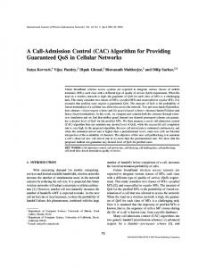
IV. N UMERICAL R ESULTS

AASP OCASP AADP OCADP

34

Probability Distribution Function

1.4

β = 3.50

1.2 1

β = 1.00

0.8 0.6 0.4 0.2 0

0

0.2

0.4

0.6

0.8

1

1.2

1.4

1.6

1.8

2

Mean Willingness to Pay per Bandwidth−Time (WTP)

1

Access Probability

0.9

β = 3.50

β = 1.00

0.8 0.7 0.6 0.5 0.4 0.3 0.2 0.1

0

0.5

1

1.5

2

2.5

Willingness to Pay (WTP) per Bandwidth−Time

Fig. 2.

WTP pdfs and access probabilities vs. price with β = 3.5 and 1.0.

Optimal Average Reward

32

30

28

26

24

22

20

18

1

1.5

Fig. 3.

2

2.5 3 3.5 Arrival Rate of Service 2

4

4.5

5

Optimal Revenue per Stage J ∗ for WTP shape β = 3.5.

350 AASP OCASP AADP OCADP

300

Number of Blocked States (Service 1)

We compare our Optimal Call Admission and Dynamic Pricing (OCADP) policy numerically with three other policies: Always Accept and Static Pricing (AASP), Optimal Call Admission and Static Pricing (OCASP) and Always Accept and Dynamic Pricing (AADP). The Always Accept component in AASP and AADP always admits a new user if sufficient bandwidth is available, which is equivalent to having no CAC at all. For both AASP and OCASP, we set the price per bandwidth time to the average price that gives access probability αPj = 0.5, j = 1, 2. For AADP and OCADP, we allow price upj and therefore αPj to vary. We purposely set up service 2 to generate higher expected revenue than service 1. The simulation parameters used are: B = 8, X = (3, 4), λn = (0.5, 1), λh = 0.25λn , 1/µ = (1, 2), σ = (0.5, 0.5), b = (1, 2), αR = (0.6, 0.6), αSO = (0.2, 0.2), αA = (0.2, 0.2) and SRj = 3rj . We will analyse the results for two WTP distributions (see Fig. 2), i.e. with β = 3.5 and 1.0. Both have the same ψ = (1, 1) per bandwidth time. As shown in Fig. 3, integrated policy OCADP generates the highest optimal expected revenue per stage, J ∗ , followed by AADP, OCASP and AASP. The reward advantage of OCADP over other policies increases as the arrival rate of service 2 increases. The optimal policy maximises revenue by exercising call admission and pricing control to: • reserve bandwidth for handoff users, • block (new) users of the lower revenue-generating service 1 to reserve bandwidth for (new) users of service 2, • set higher price per bandwidth time (and therefore lower access probability) for service 1 to discourage the arrival of its users, and • adjust prices according to the system state to encourage and discourage arrivals of all services. New users are blocked when the expected revenue gained from future-arriving handoff users exceeds that of an immediate admission of service 1 and 2 users. Similarly, service 1 users are blocked more often than of service 2 because the latter provide more expected revenue per call with higher arrival rate and call holding time. As the arrival rate of service 2 to the system increases (see Fig. 4), more service 1 users

250

200

150

100

50

0

Fig. 4.

1

2

3 Arrival Rate of Service 2

4

5

Number of States with No Admissions of Service 1 (uc1 = 0).

are blocked so that scarce system resources will only be allocated to the service that provides more revenue. However, the number of states where a service 1 user is blocked under OCADP is less than of OCASP as the latter has no control over the setting of price per bandwidth time to further influence the arrival rate of both services. In cases where network is lightly loaded, for e.g. λ = (0.5, 1), the expected average revenue generated by both services are almost the same. A typical dynamic pricing policy is illustrated in Fig. 5. The network charges higher prices per bandwidth time as the network becomes congested. Additional revenue is generated by offering below average prices per bandwidth time to users when the network is under-utilised. This result obtained is in line with the laws of demand and supply from economics which require that prices rise when demand is large relative to available supply and fall in the contrary case. A static pricing scheme that offers average, state-independent price per bandwidth time generates lower expected average revenue as it fails to offer the same incentives to users. The stationary probabilities of using AASP and OCADP are shown Fig. 6(a) and 6(b) respectively. The spikes in both graphs are due to the variation of the number of users in orbit. There is an evident displacement of probabilities from congested to less congested states when OCADP is used. The explanation for this phenomenon is simple. OCADP blocks all or some new call requests that generate lower revenue, compared to SR, and sets high prices to subsequent call admissions when the network is congested. Persistent users

0.5

0 (8,0) (7,0) (6,0) (5,0) (4,0) (3,0) (2,0) (1,0) (0,0) State of Service 2 (n2,x2)

(0,0)

(1,0)

(2,0)

(3,0)

(4,0)

(5,0)

(6,0)

(7,0)

(8,0)

State of Service 1 (n1,x1)

Fig. 5. Optimal Dynamic Pricing Policy. The x and y axes indicate the state of service 1, s1 = (n1 , x1 ), and 2, s2 = (n2 , x2 ), respectively. The combination of s1 and s2 forms a state s = (s1 , s2 ) in the system.

who are blocked or have insufficient WTP will be deferred to less congested period and therefore easing the burden on the network to always cater for the peak demand. Similar results (Fig. 7) are obtained when the probability distribution function of the WTP reduces to an exponential distribution by setting β = 1.0. However, OCASP and AASP provide lower revenue but OCADP and AADP achieve higher revenue, compared to when β = 3.5 is used. Please refer to Fig. 2 for the following explanations. The previous is due to the higher WTP placed by users with β = 1 for the same access probability αP = 0.5. In the dynamic pricing case, the average optimal access probabilities for OCADP when β = 1 ∗ and 3.5 are αP = (0.11, 0.25) and (0.13, 0.45) respectively. The higher revenue is due to the higher WTP of users at αP = 0.25 when β = 1 compared to at αP = 0.45 when β = 3.5. V. C ONCLUSIONS We have analysed a model for optimal integrated call admission and dynamic pricing in a cellular system with handoffs and price-affected new arrivals. Integrated policy OCADP has the flexibility to reject new connection requests to reserve resources for handoff users or new users who value the connection more. This strategy also provides monetary incentive to low-WTP users to access the network when the load is relatively light and allocate resources to high-WTP users when the network is relatively congested. ACKNOWLEDGMENT

0.8 0.7

Stationary Probability

1

[5] L. DaSilva, “Pricing for QoS-enabled networks: A survey,” IEEE Communications Surveys, pp. 2–8, Second Quarter 2000. [6] D. P. Bertsekas, Dynamic Programming and Optimal Control, vol. 1 and 2. Athena Scientific, Massachusetts, 1995. [7] J. Hou, J. Yang, and S. Papavassiliou, “Integration of pricing with call admission control to meet qos requirements in cellular networks.,” IEEE Trans. on Parallel and Distributed Systems, vol. 13, pp. 898–909, September 2002. [8] C. Chuah and R. Katz, “Characterizing packet audio streams from internet multimedia applications.,” in IEEE International Conference on Communications, pp. 1199–1203, April 2002. [9] A. Silva and G. Mateus, “Performance analysis for data service in third generation mobile telecommunication networks.,” in 35th Annual Simulation Symposium, pp. 227–234, April 2002. [10] M. F. Neuts and B. M. Rao, “Numerical investigation of a multiserver retrial model,” Queueing Systems, vol. 7, pp. 169–190, 1990.

0.4 0.3 0.2

(4,0) (3,0) (2,0) (1,0) (0,0)

State of Service 2 (n2,x2)

(0,0)

(1,0)

(2,0)

(3,0)

(4,0)

(5,0)

(6,0)

(7,0)

(8,0)

State of Service 1 (n1,x1)

(a)

0.8 0.7 0.6 0.5 0.4 0.3 0.2 0.1 0 (4,0) (3,0) (2,0) (1,0) (0,0)

State of Service 2 (n2,x2)

(0,0)

(1,0)

(2,0)

(3,0)

(4,0)

(5,0)

(6,0)

(7,0)

(8,0)

State of Service 1 (n1,x1)

(b) Fig. 6. Stationary Probabilities using (a) AASP and (b) OCADP respectively. 55 AASP OCASP AADP OCADP

50

45

Optimal Average Reward

[1] J. Mackie-Mason and H. Varian, “Pricing congestible network resources,” IEEE JSAC, vol. 13, pp. 1141–48, Sept 1995. [2] C. Courcoubetis, F. Kelly, and R. Weber, “Measurment-based usage charges in communication networks,” Technical Reports, Statistical Laboratory, University of Cambridge, 1997. [3] I. Paschalidis and J. Tsitsiklis, “Congestion-dependent pricing of network services,” IEEE/ACM Trans. on Networking, vol. 8, pp. 171–184, Apr 2000. [4] I. Paschalidis and Y. Liu, “Pricing in multiservice loss networks: Static pricing, asymptotic optimality, and demand substitution effects,” IEEE/ACM Trans. on Networking, vol. 10, pp. 425–437, June 2002.

0.5

0

We would like to thank Dr. Paul Chapman and Dr. Matthew Sorell for their helpful suggestions. This research is partly supported by the Smart Internet Technology CRC. R EFERENCES

0.6

0.1

Stationary Probability

Price per bandwidth time of Service 2

1.5

40

35

30

25

20

15

10

1

Fig. 7.

1.5

2

2.5 3 3.5 Arrival Rate of Service 2

4

4.5

Optimal Revenue per Stage J ∗ for WTP shape β = 1.0.

5