PHYSICS OF FLUIDS 18, 095103 共2006兲
Optimal model parameters for multi-objective large-eddy simulations Johan Meyersa兲 and Pierre Sagautb兲 Laboratoire de Modélisation en Mécanique, Université Pierre et Marie Curie, Boite 162, 4 place Jussieu, 75252 Paris cedex 05, France
Bernard J. Geurtsc兲 Multiscale Modeling and Simulation, Mathematical Sciences, J.M. Burgers Center, University of Twente, P.O. Box 217, 7500 AE Enschede, The Netherlands
共Received 21 March 2006; accepted 1 August 2006; published online 18 September 2006兲 A methodology is proposed for the assessment of error dynamics in large-eddy simulations. It is demonstrated that the optimization of model parameters with respect to one flow property can be obtained at the expense of the accuracy with which other flow properties are predicted. Therefore, an approach is introduced which allows to assess the total errors based on various flow properties simultaneously. We show that parameter settings exist, for which all monitored errors are “near optimal,” and refer to such regions as “multi-objective optimal parameter regions.” We focus on multi-objective errors that are obtained from weighted spectra, emphasizing both large- as well small-scale errors. These multi-objective optimal parameter regions depend strongly on the simulation Reynolds number and the resolution. At too coarse resolutions, no multi-objective optimal regions might exist as not all error-components might simultaneously be sufficiently small. The identification of multi-objective optimal parameter regions can be adopted to effectively compare different subgrid models. A comparison between large-eddy simulations using the Lilly-Smagorinsky model, the dynamic Smagorinsky model and a new Re-consistent eddy-viscosity model is made, which illustrates this. Based on the new methodology for error assessment the latter model is found to be the most accurate and robust among the selected subgrid models, in combination with the finite volume discretization used in the present study. © 2006 American Institute of Physics. 关DOI: 10.1063/1.2353402兴 I. INTRODUCTION
Large-eddy simulation 共LES兲 forms an emerging computational tool for the prediction of turbulent flows.1–4 The methodology combines an accurate representation of turbulent flow phenomena with a computationally affordable representation of the flow dynamics. To this end, the NavierStokes equations, which govern the flow physics, are lowpass filtered, and the effects of small-scale turbulent motions, which would require very fine grid representations in direct numerical simulations 共DNS兲, are instead incorporated using a subgrid-scale closure. At the coarse resolutions that are commonly adopted in present-day large-eddy simulations, an important problem is the intricate interaction between errors due to the subgridscale model and errors introduced by the discrete representation of the resolved-scale flow dynamics.5,6 The realization is growing that a proper understanding of the complex error dynamics, involving numerical errors and subgrid-scale modeling errors, is paramount for the credibility of LES as a valid prediction tool for turbulent flows. Various contributions have been presented recently,7–13 aiming at the identia兲
Also at: Department of Mechanical Engineering, Katholieke Universiteit Leuven. Electronic mail:
[email protected], johan.meyers@ mech.kuleuven.be b兲 Electronic mail:
[email protected] c兲 Also at: Anisotropic Turbulence, Fluid Dynamics Laboratory, Faculty of Applied Physics, Eindhoven University of Technology, P.O. Box 531, 5600 MB Eindhoven, The Netherlands. Electronic mail:
[email protected]
1070-6631/2006/18共9兲/095103/12/$23.00
fication of modeling and numerical errors, or the formulation of reliability guidelines. A central issue in the assessment of LES is the methodology which is used to identify the quality of results. Various effects can play a role which complicates the interpretation of the reliability of a simulation. Numerical discretization, specific properties of the subgrid-scale closure, the flow conditions of the selected reference case, the use of explicit filtering or de-filtering during the simulation or during postprocessing, etc., can all contribute strongly to the accumulated total simulation error. One recently proposed approach to assess LES consists of the systematic variation of simulation parameters.7,8 Such a database-analysis allows to obtain a general overview of the error behavior in the form of so-called “error landscapes.”8 Based on the systematic variation of the Smagorinsky model-parameter, the spatial resolution and the Reynolds number in LES of decaying homogeneous isotropic turbulence,8 it was demonstrated that errors resulting from such a well-known “Smagorinsky-fluid” may strongly interact with discretization errors. Moreover, “optimal refinement trajectories” were obtained, which provide the optimal model parameter, resulting in the lowest simulation error at given resolution. Later,9 these optimal refinement trajectories were compared with the predicted model-coefficient that results from the dynamic eddy-viscosity model.14 This showed that the error-landscape approach can also be very instructional in
18, 095103-1
© 2006 American Institute of Physics
Downloaded 24 Jan 2007 to 130.89.8.20. Redistribution subject to AIP license or copyright, see http://pof.aip.org/pof/copyright.jsp
095103-2
Phys. Fluids 18, 095103 共2006兲
Meyers, Sagaut, and Geurts
the interpretation of the quality other eddy-viscosity subgrid models. We recall that the error-landscape for a “Smagorinsky fluid” provides a detailed overview of a selected simulation error as function of the spatial resolution N and the Smagorinsky parameter Cs.8 Each point in the Cs-N plane corresponds to a particular large-eddy simulation which displays its own specific deviation from the exact direct numerical simulation results. An “error landscape” is created by considering the total simulation-error for a systematically varied set of Cs-N points, leading to an extensive database approach. In this error landscape the line Cˆs共N兲, for which the total simulation-error is minimal at given resolution N, represents the “optimal refinement strategy.” The present study aims to extend the error-landscape framework. The specific definition for the error that is used to identify optimal refinement trajectories can have a considerable influence on the location of these trajectories. As an example, the optimal refinement trajectory for the resolved kinetic energy is quite different from that for the resolved enstrophy. This is particularly true at coarse resolutions where the contributions from the different error sources have a significant influence. Hence, the optimization of simulation results towards one specific flow property can often imply a strongly reduced accuracy for the prediction of other flow properties. In this paper we will allow the error measure to be based on various flow properties simultaneously. In this extension we hence monitor a collection of flow quantities in a systematic way, instead of considering only one property. It is shown that for sufficiently high spatial resolutions parameter settings can be identified where all separate error measures that are included are simultaneously “near optimal.” This gives rise to so-called “multi-objective optimal parameter regions.” These regions are found to depend strongly on the Reynolds number and the spatial resolution. At too coarse resolutions, no multi-objective optimal regions may exist. In such a case the simulation can not provide an acceptably low level for all individual components in the error definition. This is indicative of a clear underresolution in which the combined effects of discretization and modeling errors express themselves in very different ways for different flow properties. Correspondingly, the reliability of a large-eddy simulation under such computational conditions is quite low. Conversely, the absence of a connected near-optimal region that results from the extended error landscape can be used as a sharp indicator for such unreliable computational settings. The identification of multi-objective optimal regions presents a framework to compare LES models. First of all, the error level in these parameter regions can be compared, thereby comparing the best results a particular model can produce. Secondly, the location of the multi-objective optimal regions of different models can be inferred. This quantifies the robustness of a particular model and also identifies the lower resolution range beneath which the reliability of a large-eddy simulation seriously deteriorates. We will consider LES to be “reliable” at certain model parameters and
numerical settings if a chosen set of flow properties is simultaneously predicted within an “acceptable” fraction of the optimum. Obviously, it is required that these monitoring quantities encompass both large-scale error measures as well as measures that characterize small-scale errors. Correspondingly, if not all monitored flow properties are properly predicted simultaneously then the adopted model and numerical parameters are considered to lie outside the multi-objective optimal region. This measure for reliability will be discussed and motivated in more detail in this paper. We will adopt this extended error-landscape analysis to the Lilly-Smagorinsky model,15 the dynamic Smagorinsky model, and a new eddyviscosity model, which results from a modification of the Smagorinsky model that is Re-consistent.16 The organization of this paper is as follows. In Sec. II we introduce the “multi-objective optimal parameter regions” and interpret their usage in terms of comparing different subgrid models. Section III is devoted to a discussion of such a comparison of the three identified eddy-viscosity models. Concluding remarks are collected in Sec. IV.
II. MULTI-OBJECTIVE OPTIMAL PARAMETER REGIONS
We first describe the setup of the simulations in Sec. II A. Then, we proceed in Sec. II B with the description of the methodology that is used to identify multi-objective optimal parameter regions. Various large- and small-scale flow properties will be incorporated in this analysis and the corresponding definition of the simulation error is clarified. A. Nomenclature and setup of the simulations
The filtered Navier-Stokes equations for incompressible flows can be written in dimensionless form as
¯Sij ij ¯ui ¯ui¯u j ¯p + − 2 − = 0; + x j x j t x j xi
i = 1,2,3
共1兲
where ¯ui is the filtered velocity component in the xi-direction, ¯p the filtered pressure and a dimensionless viscosity. Throughout, the LES filter is denoted by 共·兲, and ¯S = 关¯u / x + ¯u / x 兴 / 2 corresponds to the filtered strain ij i j j i tensor. The filtering of the convective terms gives rise to the subgrid-scale stress tensor
ij = ¯ui¯u j − uiu j .
共2兲
In large-eddy simulations, these subgrid-scale stresses are replaced by a model mij, which approximates their dynamic effect and is based on the resolved velocity field ¯ui only. One of the most often employed formulations for mij is the Smagorinsky model, given by17 ¯ 兩S ¯ = 2 ¯S , mij = 2共Cs⌬兲2兩S ij t ij
共3兲
with Cs the Smagorinsky coefficient, ⌬ the LES filter width, ¯ 兩 = 共2S ¯ ¯S 兲1/2 the magnitude of the filtered strain-rate ten兩S ij ij sor, and t the eddy viscosity related to the model. This
Downloaded 24 Jan 2007 to 130.89.8.20. Redistribution subject to AIP license or copyright, see http://pof.aip.org/pof/copyright.jsp
095103-3
Phys. Fluids 18, 095103 共2006兲
Optimal model parameters
FIG. 1. Error surfaces of LES employing the Smagorinsky model for the Re = 100 case. Errors are related to the resolved kinetic energy, i.e., ⑀E 共a兲; and to the resolved enstrophy, i.e., ⑀E 共b兲. The locations indicated by 共쎲兲 correspond to the different simulations that were included.
model will be used in the current section. Two additional models, i.e., the dynamic Smagorinsky model14 and a Re-consistent modification of the Smagorinsky model will be added and described in more detail in Sec. III. In all simulations a second-order cell-centered finitevolume method is employed to discretize the closed LES equations. This is combined with a four-stage, second-order accurate Runge-Kutta time integration. Large-eddy simulations of decaying homogeneous isotropic turbulence are carried out at a number of resolutions and different values for the model parameter Cs, and for two different Reynolds numbers, i.e., Re = 50 and 100 in terms of the TaylorReynolds number Re. The initial fields for the LES are generated by filtering the initial DNS fields8 with a cubical sharp cut-off filter, with cut-off related to the grid cut-off wavenumber kc = / h, with h the grid spacing. During the simulations, no additional explicit filtering is performed and for the implementation of the Smagorinsky model, we further take ⌬ = h.
B. Methodology for the evaluation of simulation results
In order to quantify the total simulation error in a specific large-eddy simulation, at resolution N and modelparameter Cs we turn in first instance to the relative error based on the decay of the resolved kinetic energy E共t兲 ¯ i¯ui / 2典. Here 具·典 denotes a volume averaging over the flow = 具u domain. The relative error ⑀E is given by8
⑀E共N,Cs兲 =
冤
冕
T
0
共ELES共t兲 − EDNS共t兲兲2dt
冕
T
0
2 EDNS 共t兲dt
冥
1/2
,
共4兲
with EDNS the filtered DNS energy obtained by adopting a sharp cut-off filter with kc = / h. The integration over time corresponds to approximately two eddy-turnover times. In a similar way, one can introduce an overall relative error ⑀E based on the evolution of the resolved enstrophy
Downloaded 24 Jan 2007 to 130.89.8.20. Redistribution subject to AIP license or copyright, see http://pof.aip.org/pof/copyright.jsp
095103-4
Phys. Fluids 18, 095103 共2006兲
Meyers, Sagaut, and Geurts
¯ i ¯ i / 2典 during the LES, using EDNS as a reference. Here, E = 具 ¯ = ⫻ ¯u is the filtered vorticity. In Fig. 1共a兲, the global behavior of the error ⑀E is displayed as function of the LES resolution N and the model coefficient, while Fig. 1共b兲 displays the same information for ⑀E. Both error landscapes are based on simulations at Re = 100 and include 189 different large-eddy simulations, i.e., at 21 different values for the model coefficient and 9 different resolutions. One can clearly appreciate that “optimal refinement trajectories”8 can be identified. These provide a resolution dependent Smagorinsky coefficient Cˆs共N兲 such that the error is minimal at resolution N. However, differences between both error landscapes are visible, and clearly, the resulting “optimal refinement trajectories” for E and E are not identical. Furthermore, the error levels differ considerably. As one might expect, it is easier to accurately predict the resolved kinetic energy than the resolved enstrophy. To incorporate these dependencies of the optimal refinement strategies on resolution, flow conditions, monitoring quantity, etc., it is necessary to extend the error measure. Moreover, we relax the requirement of being exactly in the optimal computational setting of one flow quantity and rather consider “near-optimal” parameter regions, but enforce these for a set of flow quantities simultaneously. The extension of the error-landscape analysis is discussed next. We introduce a “near optimal” region ⍀共⑀兲 with respect to the error measure ⑀ as
再
⍀共⑀兲 = 共N,Cs兲兩 " N,
冎
⑀共N,Cs兲 艋a . ⑀共N,Cˆs共N兲兲
共5兲
Correspondingly, at fixed resolution N, the “near optimal” region ⍀共⑀兲 is determined by all values Cs for which the resulting simulation error ⑀ is smaller than the minimal error at that resolution, multiplied by a factor a ⬎ 1. In Fig. 2共a兲, the “near optimal” region ⍀共⑀E兲 based on ⑀E 关cf. Fig. 1共a兲兴 is displayed for Re = 100. We selected the value a = 1.2 in this illustration. The optimal refinement strategy is marked at the different simulation resolutions. As can be observed from this figure, ⍀共⑀E兲 provides a clear overview of the robustness of the model, with respect to its perresolution optimal error level. At low resolutions, one can observe a fairly narrow “near optimal” region, indicating that model coefficients should be carefully selected since otherwise the total simulation error would increase strongly. At higher resolutions the “near optimal” region widens. In these cases the contribution of the subgrid model is reduced because of the reduction in ⌬ = h = 1 / N, and the flow is resolved more accurately. This allows a wider margin in specifying Cs, without exceeding the optimal error level by more than 20%. In order to determine parameter regions where more than one error is “near optimal,” one can display their respective ⍀共⑀兲 regions in one figure. In Fig. 2共b兲 this is illustrated in terms of the respective “near optimal” regions for ⑀E and ⑀E.
FIG. 2. “Near optimal” regions related to different error definitions for the standard Smagorinsky model at Re = 100. 共a兲 ⍀共⑀E兲; and 共b兲 both for ⍀共⑀E兲 and ⍀共⑀E兲. The “near optimal” regions are shaded gray and semitransparent, such that parameters in which both overlap appear with darker shades of gray. 共– –兲 and 共¯兲 respectively mark the limits of ⍀共⑀E兲 and ⍀共⑀E兲. Symbols correspond to the optimal refinement strategy for the different error definitions, where 共쎲,䉳兲 correspond respectively to ⑀E and ⑀E.
In this figure, “near optimal” regions are displayed semitransparent, such that overlapping regions appear in darker shades of gray. Hence, a region where both ⑀E and ⑀E are “near optimal” within a factor a can be simply discriminated. We will refer to such regions, corresponding to the intersection of several “near optimal” regions, as “multi-objective optimal regions.” The value a = 1.2, which was selected to construct Fig. 2, will be maintained throughout the paper. Decreasing a toward 1 implies that the “near optimal regions” shrink towards the “optimal refinement trajectory.” As a becomes low enough, there is no longer a significant overlap between different ⍀共⑀兲. The value of a and the specific measures for the error that are included in an analysis can not be characterized in general; rather this aspect is to some extent application specific. Here we will focus on a strict test for accuracy and reliability by including both large- and small-scale flow properties in the error measure. This will be introduced next. Measuring errors in large as well as small scales can be formulated in terms of specifically weighted resolved kinetic energy spectra. Two different error measures will be investi-
Downloaded 24 Jan 2007 to 130.89.8.20. Redistribution subject to AIP license or copyright, see http://pof.aip.org/pof/copyright.jsp
095103-5
Phys. Fluids 18, 095103 共2006兲
Optimal model parameters
gated which are distinguished by a superscript “a” or “b.” First we define simulation errors arising in a simulation at resolution N and model coefficient Cs as
⑀ap共N,Cs兲
=
冤
冕 再冕 冕 再冕 T
kc
0
k p共ELES共k,t兲 − EDNS共k,t兲兲dk
0
T
0
kc
k EDNS共k,t兲dk p
0
冎
2
dt
冎
2
dt
冥
1/2
.
共6兲
Here, E共k , t兲 is the resolved three-dimensional energy spectrum, which is a function of the wavenumber k and time t. Further kc = / h is the cut-off wavenumber related to the LES grid and p is a parameter, which allows to emphasize different scales in the solution. One can readily verify, based on standard relations for isotropic turbulence18,19 that
⑀a0 ⬅ ⑀E ,
共7兲
⑀a2 ⬅ ⑀E ,
共8兲
a ⑀−1 ⬅ ⑀L ,
共9兲
where L is the longitudinal integral length scale of turbulence. Hence, errors in large-scale properties are characterized by low values of p while small-scale errors require higher values of p. The formulation of the error measures ⑀ap in Eq. 共6兲 is appealing since it allows a precise interpretation in terms of well known physical quantities. However, this error definition does not correspond to a mathematical norm and may yield relatively small values even though the LES spectrum may deviate considerably from the DNS spectrum in certain wavenumber ranges. Such may occur if an overprediction of the spectrum for certain wavenumbers k is accompanied by an under-prediction at other wavenumbers. This would be considered a significant total error, but such may not be as clearly expressed by ⑀ap. An alternative error definition may be introduced which does directly connect to a mathematical norm in spectral space. This error measure is given by
⑀bp共N,Cs兲
=
冤
冕冕 T
0
kc
0
k2p兵ELES共k,t兲 − EDNS共k,t兲其2dkdt
冕冕 T
0
kc
0
2 k2pEDNS 共k,t兲dkdt
冥
1/2
,
共10兲
in which every deviation of ELES共k , t兲 from EDNS共k , t兲 is counted as a positive contribution to the total error. In contrast to ⑀ap, the error measures ⑀bp can not be interpreted in terms of common physical properties. In the sequel we will compare these different error measures and investigate their effect on the multi-objective optimal region that may be obtained. Based on the definitions for ⑀ap and ⑀bp the “multiobjective optimal regions” can now be investigated. To this end, p = −1, 0, 1, and 2 are considered for decaying homogeneous isotropic turbulence at Re = 50 and 100. In Fig. 3, near
optimal regions corresponding to the different error measures are presented. The Re = 50 case in Figs. 3共a兲 and 3共c兲 shows that if ⑀bp is used 关Fig. 3共c兲兴 a clear multi-objective optimal region emerges as the intersection of the near optimal regions for different values of p. In contrast, when using ⑀ap 关Fig. 3共a兲兴 we notice that the multi-objective optimal region may not continue to high resolutions. In particular, this arises for N 艌 60 in the specific case Re = 50. This shortcoming of the error-measure ⑀ap coincides with situations in which the effect of the model is already quite small. The specific behavior associated with ⑀ap may be related to the fact that it is not a strict norm for the energy-spectra in k-space. As a result, if ELES共k , t兲 − EDNS共k , t兲 changes sign as function of the wavenumber k, then the error-assessment based on ⑀ap will differ considerably from that based on ⑀bp. In addition, because different weights are given to different regions of k-space via the selected value for p, the effects of such signchanges are expressed differently at different resolutions. This relies on the detailed error-cancellations between modelling and discretization errors that may vary significantly with resolution.8 In Fig. 3共a兲 this cancellation expresses itself in a discontinuation of a connected multi-objective region. Multi-objective regions which are simply connected, such as arise when use is made of ⑀bp, may be preferred, and in this respect, evaluations based on ⑀ap should be handled with some caution. At Re = 100 关Figs. 3共b兲 and 3共d兲兴 the use of ⑀bp also yields a clear multi-objective optimal region over the full resolution range under consideration. Compared to the Re = 50 case, this region is shifted toward somewhat higher Cs values indicating the higher dissipation levels that are required at the same resolution, to achieve accurate results at this higher Reynolds number. In case ⑀ap is used instead we observe that also at Re = 100 the multi-objective optimal region is much more narrow. Moreover, the different near optimal regions ⍀共⑀ap兲 are observed to have no overlap for N ⬍ 48 which did not occur in the Re = 50 case. This region is indicative of too low resolution and a correspondingly reduced reliability of the simulation. The error measure ⑀ap is much more sensitive to such shortcomings than ⑀bp. This will be further elaborated based on an evaluation of the different error levels. Apart from the location of the near optimal regions ⍀共⑀ p兲 the error levels that are characteristic for these regions are of central importance. Therefore, in the following, both optimal error levels associated with ⑀ p and multi-objective optimal errors will be compared. The identification of the latter multi-objective errors at a certain resolution N requires a combination of the different error landscapes into one. This will be done with respect to a weighted overall error defined as
˜⑀共N,Cs兲 =
兺p 关⑀p共N,Cs兲/⑀p共N,Cˆs共p兲共N兲兲兴 兺p 关1/⑀p共N,Cˆs共p兲共N兲兲兴
,
共11兲
ˆ 共p兲共N兲 denotes the optimal refinement strategy assowhere C s ciated with error measure ⑀ p. Note that 共11兲 can be formu-
Downloaded 24 Jan 2007 to 130.89.8.20. Redistribution subject to AIP license or copyright, see http://pof.aip.org/pof/copyright.jsp
095103-6
Meyers, Sagaut, and Geurts
Phys. Fluids 18, 095103 共2006兲
FIG. 3. “Near optimal” regions of Smagorinsky LES related to different error definitions 共p = −1 , 0 , 1 , 2兲, with 共a,b兲 ⑀ap, and 共c,d兲 ⑀bp. Two different Reynoldsnumber cases are shown, i.e., 共a,c兲 Re = 50, and 共b,d兲 Re = 100. Different “near optimal” regions are shaded gray and semitransparent, such that regions with overlap appear with darker shades of gray. 共—兲, 共– –兲, 共–·兲, and 共¯兲 respectively mark the limits of the ⑀−1, ⑀0, ⑀1 and ⑀2 “near optimal” regions. Symbols correspond to the optimal model coefficients at the different simulation resolutions for the different error definitions, where p = −1 , 0 , 1 , 2 corresponds respectively to 共䊏,쎲,䉴,䉳兲.
lated in terms of ⑀ap and ⑀bp. This distinction will be denoted by ˜⑀a or ˜⑀b. We will define a “multi-objective optimal refinement trajectory” as the “optimal refinement trajectory” of ˜⑀. Although this identification is obviously not unique, it does provide the required characteristic indication of the total error level associated with the combination of different error landscapes. In the definition of ˜⑀, the different errors ⑀ p共N , Cs兲 are compensated with their respective optimal erˆ 共p兲共N兲兲. This ensures that error measures with rors ⑀ p共N , C s quite different levels can be combined properly. For example, errors ⑀2 which are considerably higher than ⑀−1, do not dominate the averaged error ˜⑀ because of the particular construction in 共11兲. We checked that the resulting “multiobjective optimal refinement trajectories” are situated well inside the multi-objective optimal region observed in Fig. 3. In Fig. 4, the “multi-objective optimal refinement trajec˜ 共N兲 are displayed based on ˜⑀a or ˜⑀b. Despite the tories” C s 共subtle兲 differences between these definitions of the error both result in roughly the same “multi-objective optimal re˜ b共N兲 ˜ a共N兲 and C finement trajectories.” This robustness of C s s enhances the credibility of these “optimal” Smagorinsky coefficients. Although the different near optimal regions ⍀ p
display considerable differences, their combination at various small and large values of p yields a well defined “trace” in the error landscape. We now turn to the individual error levels at p = −1, 0, 1
FIG. 4. “Multi-objective optimal refinement trajectory” based on ˜⑀a 共—兲 and on ˜⑀b 共– –兲, for both Re = 50 共䊐兲, and Re = 100 共䊊兲.
Downloaded 24 Jan 2007 to 130.89.8.20. Redistribution subject to AIP license or copyright, see http://pof.aip.org/pof/copyright.jsp
095103-7
Optimal model parameters
Phys. Fluids 18, 095103 共2006兲
FIG. 5. Errors 共p = −1 , 0 , 1 , 2兲 along their respective optimal refinement trajectories and along a multi-objective optimal refinement trajectory 共cf. Fig. 4兲 for the Re = 50 共a,c兲 and Re = 100 共b,d兲 cases using both ⑀ap 共a,b兲 and ⑀bp 共c,d兲. 共Full line and closed symbols兲: errors along the multi-objective optimal trajectory; ˆ 共p兲共N兲. 共䊏,쎲,䉴,䉳, and their open counterparts兲 correspond 共Dashed line and open symbols兲: errors along the respective optimal refinement trajectories C s a,b respectively to ⑀ p 共p = −1 , 0 , 1 , 2兲.
and 2. For completeness we compare the errors induced ˆ 共p兲共N兲 and along the multi-objective opalong the optimum C s ˜ 共N兲. This further characterizes the sensitivity of the timum C s occurring errors arising from slight variations in the Smagorinsky coefficient. In Fig. 5 the different errors are compared. We notice that ⑀2 ⬎ ⑀1 ⬎ ⑀0 ⬎ ⑀−1 at any resolution, which illustrates the well-known fact that small-scale features are more difficult to predict in large-eddy simulations. Furthermore, ⑀bp ⬎ ⑀ap which arises from the strictly positive integrands in the definition of ⑀bp, as opposed to the possible sign changes that are allowed in the integrands that define ⑀ap. For ˆ 共p兲 and both Reynolds numbers the errors ⑀bp induced along C s ˜ b are seen to correspond quite closely. A similar robustness C s is observed when the error is measured in terms of ⑀ap, but only at sufficiently high resolutions. As remarked before in relation to Fig. 3共b兲, the use of ⑀ap at coarse resolutions does not lead to a 共large兲 connected region where the different ⍀ap overlap. In Fig. 5共b兲, one can ˜ 共N兲 are not close to the errors observe that the errors along C s
along Cˆs共p兲共N兲 共p = −1 , 0 , 2兲, while they are close for Cˆs共1兲共N兲. This implies that, in terms of ⑀ap one can tune an underresolved simulation to predict one flow property optimally, but at the expense of a reduced accuracy for other flow properties. Obviously, this is connected with reduced reliability of such simulations. If errors for resolutions N ⬍ 48 are considered based on ⑀bp, one can observe this reduced reliability in a drastic increase of the error levels. Moreover, for the smallscale related errors ⑀b1 and ⑀b2 a change of slope of ⑀bp共N兲 occurs at N ⬇ 48. The differences in the respective optimal refinement strategies associated with ⑀ap are also reflected in the resolved kinetic energy spectrum. In Fig. 6 spectra are presented for the optimal solutions at N = 24 that arise in terms of ⑀a0 and ⑀a2. As can be appreciated from this figure, neither solution provides very accurate results of the energy distribution over the different wavenumbers. The more striking differences that occur are related to the under- and over-prediction of the DNS spectrum at different wavenumber intervals. In terms of
Downloaded 24 Jan 2007 to 130.89.8.20. Redistribution subject to AIP license or copyright, see http://pof.aip.org/pof/copyright.jsp
095103-8
Meyers, Sagaut, and Geurts
FIG. 6. Spectra for N = 24, t = 1.0, Re = 100, and the optimal model setting corresponding to 共–䊊–兲 ⑀a0, and 共·䉰·兲 ⑀a2. 共—兲: DNS reference solution.
⑀a0 and ⑀a2 the simulation errors may be optimal, but this is to some extent due to a partial cancelation arising from sign changes in the integrands and not so much related to predictions which actually achieve high accuracy. The wavenumber where the DNS and LES spectra intersect is seen to increase with increasing p The extended analysis of the error landscapes has so far been restricted to the Smagorinsky eddy-viscosity model. In the next section we will incorporate other eddy-viscosity models and interpret their error behavior in relation to the Smagorinsky model. We will include the popular dynamic eddy-viscosity model14,20 and a proposed modification of the Smagorinsky model. III. A COMPARISON OF ERROR DYNAMICS OF EDDY-VISCOSITY SUBGRID-SCALE MODELS
In this section we adopt the extended error-landscape analysis to quantify the error behavior of the dynamic eddyviscosity model and a modified Smagorinsky model. In Sec. III A we focus on the dynamic model and determine the near-optimal parameter regions for the modified Smagorinsky model in Sec. III B. A. Dynamic eddy-viscosity model
The dynamic procedure14,20 has been widely used in large-eddy simulations, in particular in combination with eddy-viscosity modeling, and its success can be attributed to its adaptability to a wide range of flow conditions.21 This model was shown to provide rapidly decreasing total simulation errors in the resolved kinetic energy, with increasing resolution.9 However, the error levels were observed to be a factor of two or more larger than the optimal error level. Here, we extend this database analysis and consider the suitability of the dynamic model both for large- as well as smallscale flow features. Moreover, as point of reference, a comparison with a Lilly-Smagorinsky model,15 is also presented. We closely follow the implementation of the dynamic procedure as specified in Ref. 9. The explicit test filter that is required in the dynamic procedure corresponds to a top-hat filter with filter width 4h. In Fig. 7, the dynamic model co-
Phys. Fluids 18, 095103 共2006兲
FIG. 7. Comparision of the dynamic refinement trajectory with the multiobjective trajectory based on ˜⑀a and Lilly’s Smagorinsky constant at Re = 100. 共—兲: multi-objective optimal trajectories; 共– –兲: dynamic estimation of Cs; 共–·兲: Lilly’s Smagorinsky constant.
efficient is shown as function of the resolution N at Re = 100. This is compared with Cs = 0.1733 as suggested by Lilly15 and the multi-objective refinement trajectory that was determined in the previous section. The dynamic coefficient is shown to be considerably larger than the optimal value, although also well below the Lilly-value. Correspondingly, the predictions obtained with the dynamic model are generally more accurate than those with the Lilly-Smagorinsky model. A similar result was obtained at Re = 50. We turn to the induced error levels next. In Fig. 8, the errors for p = −1, 0,1, and 2 of the dynamic Smagorinsky model are compared with the optimal level. The dynamic model is seen to result in much higher error levels, particularly in relation to small-scale flow features. A rapid reduction of the simulation error occurs only at sufficiently high resolutions. Specifically, at Re = 50 we notice that all predictions improve with increasing N while at Re = 100 a monotonously decaying error level is observed for all p only in case N 艌 48. Compared to the Lilly-Smagorinsky model the dynamic model was found to be up to about a factor two more accurate for all values of p. To further improve the correspondence between a dynamic model and the optimal parameter settings, modifications to the dynamic procedure might be considered.22–24 This line of extended dynamic procedures will be pursued in a database analysis in the future. B. Modified Smagorinsky model
In this subsection we investigate the near-optimal parameter regions and induced error levels for a proposed modification of the Smagorinsky model. The Smagorinsky model yields large-eddy simulations in which the total viscosity is given by tot = 共Cs⌬兲2兩S兩 + 关cf. Eq. 共3兲兴. As can be appreciated from results in the previous sections, the associated optimal model coefficients depend both on the Reynolds number and the simulation resolutions. Therefore, a slightly modified formulation of the total viscosity was proposed in Ref. 16, to reduce these sensitivities. We will assess the error-dynamics associated with this model
Downloaded 24 Jan 2007 to 130.89.8.20. Redistribution subject to AIP license or copyright, see http://pof.aip.org/pof/copyright.jsp
095103-9
Phys. Fluids 18, 095103 共2006兲
Optimal model parameters
FIG. 8. Comparison of the errors ⑀ap generated by the dynamic Smagorinsky model with the respective optimal errors, for Re = 50 共a兲, and Re = 100 共b兲. 共Full line and closed symbols兲: results of the dynamic procedure; 共Dashed line and open symbols兲: the respective optimal errors. 共䊏,쎲,䉴,䉳, and their open counterparts兲 correspond respectively to ⑀ap 共p = −1 , 0 , 1 , 2兲.
based on the above introduced methodology. The alteration needed to obtain the modified Smagorinsky model corresponds to
冑
¯ 兩2 + 2 , tot = 共Cs*⌬兲4兩S
共12兲
with Cs* a model coefficient. Based on a Lilly-type analysis,15 and the assumption of a cubical sharp cut-off filter, the model coefficient Cs* associated with this model theoretically corresponds to16 Cs* = 0.142. At very high Reynolds numbers Eq. 共12兲 approaches the classical Smagorinsky model. The sensitivity of these models on the optimal coefficient in the high-Re limit should be considered separately. The current approach based on having a full DNS available is then no longer applicable and one should develop more general error-assessment procedures, e.g., including theoretical properties of the turbulence at very high Re and experimental data replacing DNS as point of reference. A detailed exposition of the spectral properties of
this modified Smagorinsky model may be found in Ref. 16. Here, we restrict ourselves to the induced error-dynamics arising from this model. We will now evaluate the error behavior of the model in Eq. 共12兲, by systematically varying Cs* following the methodology in Sec. II. In Fig. 9 “near optimal regions” are displayed for p = −1, 0,1,2 and the error definition ⑀bp. Similar to what was observed for the Smagorinsky model, connected near-optimal parameter regions ⍀共⑀ p兲 may be distinguished. Compared to the Smagorinsky model, the modified model results in considerably more extended near-optimal regions which quantifies that the new model is less sensitive to variations in the model-parameter. Moreover, the horizontal line corresponding to the value Cs* = 0.142 appears to be in the overlap of all these near-optimal regions for virtually all resolutions. This can be an important advantage as it greatly facilitates the a priori estimation of a resolution-independent
FIG. 9. “Near optimal” regions of the modified Smagorinsky LES related to different error definitions 共p = −1 , 0 , 1 , 2兲, with Re = 50 共a兲, and Re = 100 共b兲. Different “near optimal” regions are shaded gray and semitransparent, such that regions with overlap appear with darker shades of gray. 共—兲, 共– –兲, 共–·兲, and 共¯兲 respectively mark the limits of the ⑀−1, ⑀0, ⑀1 and ⑀2 “near optimal” regions. Symbols correspond to the optimal model coefficients at the different simulation resolutions for the different error definitions, where ⑀ p 共p = −1 , 0 , 1 , 2兲 corresponds respectively to 共䊏,쎲,䉴,䉳兲.
Downloaded 24 Jan 2007 to 130.89.8.20. Redistribution subject to AIP license or copyright, see http://pof.aip.org/pof/copyright.jsp
095103-10
Phys. Fluids 18, 095103 共2006兲
Meyers, Sagaut, and Geurts
FIG. 10. Errors ⑀ap 共p = −1 , 0 , 1 , 2兲 along their respective optimal refinement trajectories and along Cs = 0.1420 for the Re = 50 共a,c兲 and Re = 100 共b,d兲 cases and for both the standard Smagorinsky model 共a,b兲 and the modified Smagorinsky model 共c,d兲. 共Full line and closed symbols兲: along Cs = Cs,ref ; 共Dashed line and open symbols兲: along the respective optimal refinement trajectories. 共䊏,쎲,䉴,䉳, and their open counterparts兲 correspond respectively to ⑀ p 共p = −1 , 0 , 1 , 2兲.
model coefficient which is close to the multi-objective optimal parameter region. We finally turn our attention to the induced error levels 共Fig. 10兲. If we compare the error levels of both the Smagorinsky and the modified Smagorinsky models along their optimal refinement trajectories then quite similar accuracy is observed. Moreover, if the errors of the modified model are evaluated along the constant-coefficient trajectory Cs* = 0.142, it is observed that they are very close to the overall minimal errors. This may be seen in Figs. 10共c兲 and 10共d兲. In fact, for both Reynolds numbers, and N 艌 48, the trajectory Cs* = 0.142 effectively is a multi-objective optimal refinement trajectory. While this is not anymore the case for N ⬍ 48, even here, errors are lower than those observed in the standard Smagorinsky model 关operated with Cs = 0.142, cf. Figs. 10共a兲 and 10共b兲兴 or the dynamic Smagorinsky model 共cf. Fig. 8兲. Thus, the modified model appears not only more robust, but also more accurate.
IV. CONCLUSIONS
In the present study, “near optimal parameter regions” and “multi-objective optimal parameter regions” were introduced. These definitions represent for each resolution, a band of model-coefficients where large-eddy simulations are either near optimal for the prediction of a single flow property, or, near optimal for the prediction of multiple flow properties at the same time. In the analysis two distinct error measures were introduced and compared, i.e., ⑀ap 关cf. Eq. 共6兲兴 and ⑀bp 关cf. Eq. 共10兲兴. The parameter p in these definitions can be varied such that different scales in the turbulent solution are emphasized more in the resulting error definitions. The error-measures ⑀ap may be directly identified with errors in well-known physical a properties of a flow. For example, ⑀−1 corresponds to the error in the integral length scale L, ⑀a0 to the error in the resolved kinetic energy E, and ⑀a2 provides the error in the resolved enstrophy E. In contrast, ⑀bp may not be directly
Downloaded 24 Jan 2007 to 130.89.8.20. Redistribution subject to AIP license or copyright, see http://pof.aip.org/pof/copyright.jsp
095103-11
Phys. Fluids 18, 095103 共2006兲
Optimal model parameters
interpreted in terms of errors in physical properties, but it is formulated in terms of mathematical norms. Correspondingly, this error-measure is more strict and penalizes both over- and under-predictions in the spectrum. Comparing predicted near optimal parameter regions and multi-objective optimal parameter regions based on ⑀a or ⑀b we observed larger, connected regions when ⑀b was used. Conversely, the use of ⑀a appears to yield a more sharply defined indicator for too coarse LES resolutions. When combining different near-optimal parameter regions at different p, both error definitions provide comparable “multi-objective optimal refinement trajectories.” Hence, despite the differences between ⑀a and ⑀b the desired approximation of “well motivated” parameter settings in the Smagorinsky model was found to be quite robust and not very sensitive to the use of either error-measure. We observed that in some cases a connected multiobjective optimal parameter region also ceased to exist at fairly high resolutions. In these situations the influence of the subgrid model was quite low and the predictions not very much different from well resolved DNS. Hence, at high resolutions some uncertainty might arise when trying to approximate parameters that yield the optimal relative error, particularly in combination with ⑀a. However, as the actual absolute error that occurs in these cases was found to be quite acceptable, this uncertainty at high resolutions is of little consequence. For LES of decaying homogeneous isotropic turbulence using the Smagorinsky model and a second-order cellcentered finite-volume discretization, it was shown that multi-objective optimal model settings exist for a wide range of simulation resolutions at both Reynolds numbers considered. It was further illustrated that the Lilly-Smagorinsky model and, to a lesser degree, the dynamic Smagorinsky model both employ coefficients which are well outside these multi-objective optimal regions. Consequently, both versions of the Smagorinsky model generate simulation errors which are considerably higher than potentially possible for the present test case. A direct optimization of the Smagorinsky constant might be attempted to efficiently approximate the optimal refinement strategy. However, a more straightforward improvement of the error-behavior may be obtained when use is made of a slightly modified Re-consistent Smagorinsky model. To further illustrate the presented framework for LES error assessment, a comparison between the standard Smagorinsky model and the Re-consistent eddy-viscosity model was carried out. It was shown that errors in the respective multi-objective optimal regions were virtually the same for both models. However, the new eddy-viscosity model, which corresponds to a simple modification of the Smagorinsky model, provided a much easier way to select a priori a multiobjective optimal model coefficient. In fact, the new eddyviscosity model, operated with a theoretically determined coefficient, provided LES results which were more accurate than either the standard or the dynamic Smagorinsky model. The use of homogeneous isotropic turbulence is a natural first test case for any new LES method. In this respect, the current framework for error evaluation seems to be very
promising for comparison of LES models and the numerical discretization schemes used for their implementation. As demonstrated, this can reveal interesting features specific to the model, such as its dependence on resolution and Reynolds number, while the extent of multi-objective optimal regions can also be indicative for the selection of minimal simulation resolutions. LES reliability should be obviously evaluated based on a range of test cases. Hence, the extension of the presented methodology to more complicated test cases, involving flow inhomogeneities, or more complex physical features, is an important topic of further research. In a first step, we would consider extensions towards a mixing layer or a channel flow. These test configurations have only one nonhomogeneous direction. Correspondingly, not only the average level of the model coefficient is important, but also its distribution in the non-homogeneous direction. Finding the optimal dependence of the model coefficient as function of the non-homogeneous direction is not feasible with the brute-force approach applied in the present paper, but instead gradient-based or adjoint-based optimization techniques might be envisaged. Clearly, the question of reliability, usability and robustness of a model in such a flow case should in that case also be related to the dependence or independence of its optimal model parameters to the inhomogeneous direction. If large-eddy simulations of complex applications are considered, the current approach to the evaluation of errors is no longer feasible. The required simulation times needed for such complex cases often only allow a few parameter variations. However, the present framework, and possible extensions towards other generic cases, can provide invaluable insight into the parameter regions in which models combined with their actual numerical implementation, can produce reliable results. Based on a physical understanding of the complex flow application, which can be partially obtained using several test simulations of the full-scale application, this can support the set-up of reliable and accurate simulations. The present work provides a first illustration in this direction, e.g., expressed by guidelines that quantify minimal resolutions beyond which simply connected multi-objective regions exist. Of course, further developments are needed before this may yield a reliable and practical guideline for LES of flows of realistic complexity. 1
R. S. Rogallo and P. Moin, “Numerical simulations of turbulent flows,” Annu. Rev. Fluid Mech. 16, 99 共1984兲. 2 M. Lesieur and O. Métais, “New trends in large-eddy simulations of turbulence,” Annu. Rev. Fluid Mech. 28, 45 共1996兲. 3 P. Sagaut, Large Eddy Simulations for Incompressible Flows 共Springer, Berlin, third ed., 2006兲. 4 B. J. Geurts, Elements of Direct and Large-Eddy Simulation 共Edwards, Flourtown, 2003兲. 5 S. Ghosal, “An analysis of numerical errors in large-eddy simulations of turbulence,” J. Comput. Phys. 125, 187 共1996兲. 6 B. Vreman, B. Geurts, and H. Kuerten, “Comparison of numerical schemes in large-eddy simulations of the temporal mixing layer,” Int. J. Numer. Methods Fluids 22, 297 共1996兲. 7 B. J. Geurts and J. Fröhlich, “A framework for predicting accuracy limitations in large eddy simulations,” Phys. Fluids 14, L41 共2002兲. 8 J. Meyers, B. J. Geurts, and M. Baelmans, “Database-analysis of errors in large-eddy simulation,” Phys. Fluids 15, 2740 共2003兲.
Downloaded 24 Jan 2007 to 130.89.8.20. Redistribution subject to AIP license or copyright, see http://pof.aip.org/pof/copyright.jsp
095103-12 9
Phys. Fluids 18, 095103 共2006兲
Meyers, Sagaut, and Geurts
J. Meyers, B. J. Geurts, and M. Baelmans, “Optimality of the dynamic procedure for large-eddy simulations,” Phys. Fluids 17, 045108 共2005兲. 10 M. Klein, “An attempt to assess the quality of large eddy simulations in the context of implicit filtering,” Flow, Turbul. Combust. 75, 131 共2005兲. 11 S. A. Jordan, “A priori assessments of numerical uncertainty in large-eddy simulations,” ASME J. Fluids Eng. 127, 1171 共2005兲. 12 F. K. Chow and P. Moin, “A further study of numerical errors in largeeddy simulations,” J. Comput. Phys. 184, 366 共2003兲. 13 G. De Stefano and O. V. Vasilyev, “‘Perfect’ modeling framework for dynamic SGS model testing in large eddy simulation,” Theor. Comput. Fluid Dyn. 18, 27 共2004兲. 14 M. Germano, U. Piomelli, P. Moin, and W. H. Cabot, “A dynamic subgridscale eddy viscosity model,” Phys. Fluids A 3, 1760 共1991兲. 15 D. K. Lilly, “The representation of small-scale turbulence in numerical simulation experiments,” in Proceedings of the IBM Scientific Computing Symposium on Environmental Siences 共IBM Data Processing Division, White Plains, New York, 1967兲. 16 J. Meyers and P. Sagaut, “On the model coefficients for the standard and the variational multi-scale Smagorinsky model,” J. Fluid Mech. 共to be published兲.
17
J. Smagorinsky, “General circulation experiments with the primitive equations: I. The basic experiment,” Mon. Weather Rev. 91, 99 共1963兲. 18 S. B. Pope, Turbulent Flows 共Cambridge University Press, Cambridge, UK, 2000兲. 19 G. K. Batchelor, The Theory of Homogeneous Turbulence 共Cambridge University Press, Cambridge, UK, 1953兲. 20 D. K. Lilly, “A proposed modification of the Germano subgrid-scale closure method,” Phys. Fluids A 4, 633 共1992兲. 21 S. B. Pope, “Ten questions concerning the large-eddy simulation of turbulent flows,” New J. Phys. 6, 35 共2004兲. 22 C. Meneveau and T. S. Lund, “The dynamic Smagorinsky model and scale-dependent coefficients in the viscous range of turbulence,” Phys. Fluids 9, 3932 共1997兲. 23 F. Porté-Agel, C. Meneveau, and M. B. Parlange, “A scale-dependent dynamic model for large-eddy simulation: application to a neutral atmosoheric boundary layer,” J. Fluid Mech. 415, 261 共2000兲. 24 E. Bou-Zeid, C. Meneveau, and M. Parlange, “A scale-dependent Lagrangian dynamic model for large eddy simulation of complex turbulent flows,” Phys. Fluids 17, 025105 共2005兲.
Downloaded 24 Jan 2007 to 130.89.8.20. Redistribution subject to AIP license or copyright, see http://pof.aip.org/pof/copyright.jsp