Near-Optimal Regularization Parameters for ... - Semantic Scholar

Near-Optimal Regularization Parameters for Applications in Computer Vision Changjiang Yang, Ramani Duraiswami and Larry Davis Computer Vision Laboratory University of Maryalnd College Park, MD 20742, USA

Abstract Computer vision requires the solution of many ill-posed problems such as optical flow, structure from motion, shape from shading, surface reconstruction, image restoration and edge detection. Regularization is a popular method to solve ill-posed problems, in which the solution is sought by minimization of a sum of two weighted terms, one measuring the error arising from the ill-posed model, the other indicating the distance between the solution and some class of solutions chosen on the basis of prior knowledge (smoothness, or other prior information). One of important issues in regularization is choosing optimal weight(or regularization parameter). Existing methods for choosing regularization parameters either require the prior information on noise in the data, or are heuristic graphical methods. In this work we apply a new method for choosing near-optimal regularization parameters by approximately minimizing the distance between the true solution and the family of regularized solutions. We demonstrate the effectiveness of this approach for the regularization on two examples: edge detection and image restoration.

1. Introduction Computer vision consists of the problems such as edge detection, motion estimation, surface reconstruction, and shape from shading, that aim at recovering the physical properties of surfaces in 3D from 2D images. As pointed out by Poggio et al. [11, 1] many problems of computer vision are ill-posed in the sense of Hadamard, for which at least one of the conditions of existence, uniqueness or continuity of the solution are violated. The regularization technique is a popular method to transform the original ill-posed problem to a well-posed one. The basic idea of regularization is to find an optimal approximation of the exact solution from a family of approximate solutions depending on a positive parameter called regularization parameter. The regularization param-

eter controls the degree of regularity and the closeness of the solution to the data. The choice of the value of the regularization parameter is a crucial and difficult problem in the theory of regularization. Several methods have been developed to find the regularization parameter. The discrepancy principle requires a precise estimate of the energy of the noise. The estimate of the regularization parameter is the value such that the discrepancy of the corresponding regularized solution is just equal to the energy of the noise. Another approach proposed by Miller [8] assumes that one has both a bound on the energy and a bound on the discrepancy of the unknown object. An approximate solution can be found from the intersection of the permissible regions of the two bounds. The methods considered previously require knowledge of the noise level. On the other hand, based on stochastic assumptions, generalized cross-validation (GCV) tries to choose the regularization parameter from the data itself using statistical methods [2]. The L-curve method, introduced by Hansen and O’Leary [6], is a graphical method that does not require information about the noise. The corner of the L-curve corresponds to the best compromise between approximation error and the noise-propagation error. All these regularization parameter choosing methods are either computationally intensive (as they require solution of the problem for many values of the regularization parameter), or graphically motivated (thus needing human interpretation). Recently a near-optimal method was proposed by O’Leary [9]. This method is distinguished by the fact that without the priori information about the noise, it chooses a near optimal regularization parameter which approximately minimizes the distance from the noise-free solution to the family of the regularized solutions. Compared with other methods, the computation overhead is relatively low. In this work we applied the algorithm to regularization of vision problems for determining the regularization parameter. We also extend the algorithm to the problems with general regularization term. The rest of this paper is organized as follows. In section 2 the regularization for some applications in computer vision are described. In section 3 we

explain the basic idea of the method and how it is extended to general regularization cases. In section 4, we illustrate how the method works by two specific examples. Section 5 gives the conclusion and future works.

2. Regularization of Computer Vision Regularization is quite popular in computer vision, and many ill-posed problems in computer vision can be formulated and solved as particular instances. Regularization theory was developed to provide an optimal solution from a family of admissible solutions by introducing suitable prior knowledge. Due mainly to Tikhonov [13], the regularization of the ill-posed problem of determining x from the data b: Ax = b

2.2. Image Restoration Image restoration is a task of recovering an image that has been degraded by blur and noise. An image degraded by blurring and additive noise can be modeled by a Fredholm integral equation of the first kind: ZZ g(u, v) = h(u, v; s, t)f (s, t) + n(u, v) where g(u, v) is the recorded degraded image, f (u, v) is the original true image, h(u, v) is the blurring kernel or point spread function (PSF), n(u, v) is the additive noise introduced during image acquisition. In order to restore the deblurred image Phillips [10] proposed to minimize the functional

(1)

kg − Hf k2 + λk∇2 f k2

consists of minimizing the functional: Φλ (x) = kAx − bk2 + λkLxk2

(2)

2.3. Computing Optical Flow

or equivalently, ∗

∗

∗

(A A + λL L)x = A b

(3)

where λ > 0 is a regularization parameter, L is a regularization operator chosen to obtain a solution with desirable properties such as smoothness. Many problems in computer vision can be regularized by the Tikhonov regularization theory. We will explain how it works by some applications in computer vision.

2.1. Edge Detection Edge detection is an important preprocessing step in computer vision. Torre and Poggio considered edge detection as a problem of numerical differentiation of images which is an ill-posed problem [14]. The typical procedure for the regularization of edge detection consists of two steps. In the first step data is approximated by a differentiable local function, while in the second step the derivative of the regularized approximation function is computed. Consider a 2D image g(x, y) = f (x, y) + ²(x, y), where g(x, y) is the data and ² represents error in the measurement. We want to correctly estimate f so we can choose a stabilizing operator ZZ 2 kLf k = |∇2 f |2 dxdy where ∇2 is the Laplacian. The approximation function f is the function that minimizes the functional ZZ X (g − f (x, y))2 + λ |∇2 f |2 dxdy with λ > 0.

with λ > 0.

The goal of optical flow techniques is to compute an approximation of the the 2D motion field from a sequence of images. The most commonly applied constraint is gradient constraint equation: Ex u + Ey v + Et = 0 where Ex , Ey and Et are the partial derivatives of image brightness pattern E = E(x, y, t) with respect to x,y and t respectively. To obtain a unique optical flow, Horn and Schunck [7] proposed to minimize the functional ZZ (Ex u + Ey v + Et )2 + λ(k∇uk2 + k∇vk2 )dxdy with λ > 0 and the integral is over the whole image plane.

3. Choosing Near-Optimal Regularization Parameter We first consider the standard form of Eq.(3) in which L is the identity operator. Let us denote the singular value decomposition of A as A = U ΣV ∗ where U and V have orthonormal columns and Σ is a diagonal matrix. Therefore Eq.(3) can be written as (Σ∗ Σ + λI)z = Σ∗ β

where z = V ∗ x and βi = u∗i b. Here ui is the ith column of U . Thus, the Tikhonov solution is n X σ¯i βi xλ = 2 + λ vi σ i=1 i

(4)

where vi is the ith column of V . The true solution to the discrete (noise-free) problem is xtrue =

n X βi − ²i i=1

σi

vi

(5)

where ²i = vi∗ (b − btrue ) represents the unknown noise component. Note that Eq.(5) shows that if the matrix has vanishing singular values σi ,or ones that are close to zero, the solution will exhibit ill-posed behavior. The goal in regularization is to produce a solution as close as possible to the true solution, so let us define 2

f (λ) = kxλ − xtrue k

and minimize the distance between the regularized solution and the true solution with respect to λ ¯2 n ¯ X ¯ σ¯i βi βi − ²i ¯¯ ¯ min f (λ) = min ¯ σ 2 + λ − σi ¯ λ λ i i=1 Setting the derivative of f (λ) equal to zero yields n n ¯ X X βi2 λ βi ²i + βi ²¯i 1 0 f (λ) = − =0 2 3 2 (σi + λ) 2(σi2 + λ)2 i=1 i=1 (6) The first summation in Eq.(6) is numerically computable, but the second is not because the noise values ²i are unknown. In most cases, the system satisfies the discrete Picard condition, which means that for large enough n, the sequence of true values {|βi − ²i |}, on the average, decays to zero faster than the sequence of singular values {σi } [5]. Hence for terms with i greater than or equal to some k, ²i ≈ βi , and we can compute an approximation of the function g(λ) as ! Ãk−1 n n X X X β¯i ²i + βi ²¯i βi2 λ βi2 gˆ(λ) ≡ − −E (σi2 + λ)3 (σi2 + λ)2 2(σi2 + λ)2 i=1 i=1

g(λ) ≡

i=k

where the last term denotes the expected value of the quantity. Under the assumption that the signal and the noise are independent, we have E(β¯i ²i ) = E(βi ²¯i ) = E(²2i ) = s2 , and gˆ(λ) =

n X i=1

n

k−1

X X βi2 1 βi2 λ − −s2 2 2 2 3 2 (σi + λ) (σi + λ) (σi + λ)2 i=1 i=k

As λ increases from zero, this function is monotonically increasing. Finding the zero of this function yields an approximation to the optimal value of the regularization parameter

λ. In [9] it has been shown that the regularized solution with this λ converges to the correct solution as the deviation of the noise tends to zero if the parameter k is chosen such that ²i ≈ βi for i ≥ k.

3.1. Transformation to Standard From In many applications of computer vision, regularization in standard form is not the best choice; i.e., L 6= I in problem (2). This is because the regularization may be with respect to a prior model, or may require more stringent smoothness constraints (e.g., elasticity constraints). To overcome this limitation in [9], we need to transform Eq.(2) into the following standard-form problem: ¯x − ¯bk2 + λk¯ min kA¯ xk2 For the simple case where L is square and invertible, the transformations A¯ = AL−1 , ¯b = b, x ¯ = Lx accomplish this task. The inverse transformation is x = L−1 x ¯. In most applications, the matrix L is not square or invertible, what we need is the A-weighted generalized inverse of L, denoted L†A [3]. To obtain a numerically stable algorithm, we compute the generalized singular value decomposition of the matrix pair (A, L): µ ¶ Σ 0 A=U X −1 L = V (M, 0)X −1 , 0 I and

Σt Σ + M t M = I.

Then L†A can be expressed as µ −1 ¶ M † LA = X VT 0 ¯ ¯b in this case take the form The standard-form terms A, A¯ = AL†A , where x0 =

¯b = b − Ax0 , n X

uTi bxi

i=p+1

is the unregularized component of x which is not affected by the regularization scheme. The transformation of the solution is x ¯ = L(x − x0 ) and the back transformation is x = L†A x ¯ + x0

3.2 Regularization and Filtering The regularized solution takes a very simple form in the case where A is a convolution operator. If we assume periodic boundary condition, the matrix A and L are both blockcirculant-circulant-block (BCCB) matrices in the 2D case

[4], which can be diagonalized very efficiently using fast Fourier transforms (FFTs). Suppose A = W ΣW −1 and L = W ΩW −1 , where W is the unitary discrete Fourier transform matrix, Σ and Ω are diagonal matrices. The regularized solution takes a similar form as Eq.(4) xλ =

n X i=1

σ¯i βi wi σi2 + λωi2

where wi is the ith column of W . By similar analysis, finding the zero of the function gˆ(λ) =

(a)

(b)

(c)

(d)

(e)

(f)

(g)

(h)

n X ω 2 [ω 2 (β 2 − α2 )λ − σ 2 α2 ] i

i=1

i

i

i

i

i

(σi2 + λωi2 )3

yields an approximation for the optimal value of λ, where αi = s, i < k and αi = βi , i ≥ k.

4. Experimental Results In this section we apply the algorithm to edge detection and image restoration on both synthetic and real data.

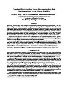
4.1. Edge Detection We use the same experimental method as in [12] to test our algorithm. The original image was first smoothed by a 2D Gaussian function then regularized by Laplacian operator. We can compute a near-optimal regularization parameter λ from the image. Then as suggested in [12], we use Canny’s edge detector with the same half amplitude in the frequency domain to test the results. Fig. 1 shows several examples of edge detection by Canny’s detector with the scales computed by regularization method. We can see that the algorithm adjust the scale of the edge detector based on the complexity of the content in the images.

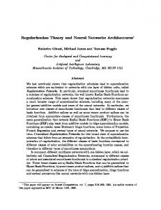
4.2. Image Restoration For the experiments of this section we restore an image distorted by spatially invariant Gaussian blur followed by the addition of white Gaussian noise. The original cameraman image is a 256×256 image. The degraded images were created by convolving the Gaussian PSF with scale 1.0 and 1.5 pixels. Normally distributed random noise was added, scaled so that the noise level was 0.01 and 0.05 times the norm of the original image. The restored images are regularized by identity operator and shown in Fig. 2. From the results, we can see that the regularization parameter correctly adjust the degree of the regularization based on the blur and the noise level.

Figure 1. Edge detection experiment: (a)original image of blood cells, (b)edges detected by Canny’s detector with σ = 1.2896, corresponding λ = 2.7659, (c)original image of Saturn, (d)edges detected by Canny’s detector with σ = 1.8968, corresponding λ = 12.9458, e)original image of circuit board, (f)edges detected by Canny’s detector with σ = 0.7333, corresponding λ = 0.2892, g)original image of bone marrow, (h)edges detected by Canny’s detector with σ = 0.5026, corresponding λ = 0.0638.

5. Conclusions

(a)

(b)

In this paper, we present a method for choosing a nearoptimal regularization parameters for the applications in computer vision. Without prior knowledge of the noise in the observation, it chooses the regularization parameter by approximately minimizing the distance between the regularized solution and the noise-free solution. If the problem is too large to directly compute, the idea can be applied by the iterative method. In the future, we will study how this method is applied to the large scale non-linear problem more efficiently.

References

(c)

(d)

(e)

(f)

(g)

(h)

Figure 2. Image restoration experiment: (a)image degraded by 1-pixel blur and 0.01 additive noise, (b)restored image with λ = 0.0068, (c)image degraded by 1-pixel blur and 0.05 additive noise, (d)restored image with λ = 0.0414, (e)image degraded by 1.5-pixel blur and 0.01 additive noise, (f)restored image with λ = 0.0031, (g)image degraded by 1.5pixel blur and 0.05 additive noise, (h)restored image with λ = 0.0180.

[1] M. Bertero, T. Poggio, and V. Torre. Ill-posed problems in early vision. Proceeding of the IEEE, 76(8):869–889, 1988. [2] P. Craven and G. Wahba. Smoothing noisy data with spline functions: Estimating the correct degree of smoothing by the methods of generalized cross-validation. Numer. Math., 31:377–403, 1979. [3] L. Elden. A weighted pseudoinverse, generalized singular values, and constrained least squares problems. BIT, 22:487–501, 1982. [4] R. C. Gonzalez and R. E. Woods. Digital Image Processing. Addison-Wesley, Reading, MA, USA, 1992. [5] P. C. Hansen. Rank-Deficient and Discrete Ill-Posed Problems: Numerical Aspects of Linear Inversion. SIAM, Philadelphia, 1998. [6] P. C. Hansen and D. P. O’Leary. The use of the L-curve in the regularization of discrete ill-posed problems. SIAM Journal on Scientific Computing, 14(6):1487–1503, Nov. 1993. [7] B. K. P. Horn and B. G. Schunck. Determining optical flow. Artificial Intelligence, 17:185–204, 1981. [8] K. Miller. Least squares methods for ill-posed problems with a prescribed bound. SIAM J. Math. Anal., 1:52–74, 1970. [9] D. P. O’Leary. Near-optimal parameters for tikhonov and other regularization methods. SIAM J. Scientific Computing, to appear. [10] D. L. Phillips. A technique for the numerical solution of certain integral equation of the first kind. J. Assoc. Comput. Machinery, 9(1):84–97, 1962. [11] T. Poggio, V. Torre, and C. Koch. Computational vision and regularization theory. Nature, 317:314–319, 1985. [12] T. Poggio, H. Voorhees, and A. Yuille. A regularized solution to edge detection. Technical Report AI-Memo-883, MIT, 1985. [13] A. N. Tikhonov and V. Y. Arsenin. Solution of Ill-posed Problems. Winston & Sons, Washinton DC, 1977. [14] V. Torre and T. Poggio. On edge detection. IEEE Trans. Pattern Anal. Machine Intell., 8:147–163, 1986.