1
Optimal Parsing Trees for Run-Length Coding of Biased Data Sharon Aviran, Paul H. Siegel, Fellow, IEEE, and Jack K. Wolf, Fellow, IEEE
Abstract— We study coding schemes which encode unconstrained sequences into run-length-limited (d, k)-constrained sequences. We present a general framework for the construction of such (d, k)-codes from variable-length source codes. This framework is an extension of the previously suggested bit stuffing, bit flipping and symbol sliding algorithms. We show that it gives rise to new code constructions which achieve improved performance over the three aforementioned algorithms. Therefore, we are interested in finding optimal codes under this framework, optimal in the sense of maximal achievable asymptotic rates. However, this appears to be a difficult problem. In an attempt to solve it, we are led to consider the encoding of unconstrained sequences of independent but biased (as opposed to equiprobable) bits. Here, our main result is that one can use the Tunstall source coding algorithm to generate optimal codes for a partial class of (d, k) constraints. Index Terms— Bit stuffing, (d, k) constraints, Optimal (d, k)codes, Parsing trees, Source Coding.
I. I NTRODUCTION A binary sequence satisfies a run-length-limited (d, k) constraint if it has the following two properties: successive ones are separated by at least d zeros and the number of consecutive zeros does not exceed k. Such sequences are called (d, k)sequences and have found widespread use in magnetic and optical recording [1]. In constrained-code design, we typically model the unconstrained user-data as a stream of independent equiprobable bits. An important, but not the only, design goal is converting such inputs into constrained sequences with high efficiency. Here, efficiency relates to asymptotic encoding rates, where the rate R of a (d, k)-code is defined as the ratio of the average input length and the average output length. The emphasis in this paper is on designing efficient (d, k)codes. The rate is evaluated with respect to the Shannon capacity of the (d, k) constraint, a measure which was shown by Shannon to equal the maximum rate achievable by any (d, k)-code [2]. It is an established result [2], [1] that for any admissible (d, k) pair the capacity exists and is given by C(d, k) = log2 λd,k , where λd,k is the largest real root of the constraint’s characteristic polynomial. The most efficient code is thus a code whose rate equals the capacity. We say that such a code achieves capacity or is capacity-achieving. This research was supported in part by NSF Grant CCR-0219582, part of the Information Technology Research Program and by the CMRR at UCSD. The material in this paper was presented in part at the IEEE International Symposium on Information Theory, Seattle, USA, July, 2006. The authors are with the Department of Electrical and Computer Engineering and the Center for Magnetic Recording Research, University of California, San Diego, La Jolla, CA 92093, USA (e-mail:
[email protected];
[email protected];
[email protected]).
The central theme of this work is twofold: a study of prior (d, k)-code constructions from a source coding perspective and the construction of new (d, k)-codes based on variable inputlength (VL) source codes. The idea of constructing (d, k)codes from source codes is not new. Numerous constructions have arisen from the following duality between constrained coding and source coding. One first models the constrained stream as a structured source from which redundancy can be removed to form unconstrained and nearly Bernoulli(1/2)distributed output. By reversing a source encoder-decoder pair, the decoder of a suitable source code is used to encode unconstrained Bernoulli(1/2)-distributed input into constrained sequences, in a recoverable manner. Applications to (d, k)code design include the adaptation of arithmetic coding techniques [3], pioneered by Martin, Langdon, and Todd. An interesting work by Kerpez [4] derives three (d, k)-codes from a Huffman code [5], a Tunstall code [5], [6], and an enumerative code [7]. The rates of the four above-mentioned constructions were shown to converge to the (d, k) capacity with increasing block length. In these designs, the choice of source code is guided by special properties of (d, k)sequences with maximum-entropy (maxentropic) distribution. Such sequences are desirable as they correspond to maximizing the code rate [2]. It is well-known that they can be parsed into a concatenation of binary strings from the set Γd,k = {0d 1, 0d+1 1, · · · , 0k−1 1, 0k 1}, where 0t stands for a run of t consecutive 0’s and where the strings are statistically independent and identically distributed (i.i.d.) [2], [1]. From now on, we refer to the strings in Γd,k as constrained phrases. The constrained-phrase maxentropic distribution is −(d+1) −(d+2) −(k) −(k+1) given by Λd,k = (λd,k , λd,k , · · · , λd,k , λd,k ), −i i−1 where λd,k is the probability of 0 1 [8]. The source code then serves as a distribution transformer (DT) between Λd,k and a Bernoulli(1/2) distribution. The (d, k)-code thus applies the inverse transformation so as to induce Λd,k on the output. An alternative design approach emerges from the literature on lossless coding of i.i.d. sources for transmission over noiseless, memoryless channels with unequal symboltransmission costs. One can accommodate (d, k)-codes into this framework by modelling (d, k)-sequences as the inputs to a memoryless channel [1]. This approach is closely related to our work and is much less investigated. Existing literature is mainly concerned with two types of codes: fixed-to-variable length and variable-to-fixed length, the latter being sparsely studied [5]. The most relevant work on fixed-to-variable length codes is a recent algorithm, which efficiently finds a prefixcode of minimum average transmission cost per source symbol
2
when the costs are integers [9]. An application to (d, k)codes is straightforward and appears in [9]. As for variableto-fixed length codes, Lempel, Even, and Cohn [10] derived an algorithm for constructing a prefix-free code of minimum average transmission cost per source symbol when the source symbols are equiprobable. It is interesting to note that both papers do not view the problem from an information-theoretic standpoint, but rather treat it from a combinatorial optimization perspective. As such, they are not concerned with maxentropic distributions. Our work relates to variable-to-fixed length codes, but relaxes the equiprobable source assumption. This work builds upon three prior (d, k)-code constructions: the bit stuffing (BS), bit flipping (BF), and symbol sliding (SS) algorithms [11], [12], [13], [14]. In all constructions, the input sequences are first fed into a binary DT. The DT preserves the bitwise independence, but results in bits that are biased towards one of two values, i.e., they constitute an i.i.d. Bernoulli(p)-distributed source. As these sequences are still unconstrained, they undergo additional processing by a constrained encoder. It is this component which varies among the algorithms. Note that although one can directly (d, k)-encode the standard equiprobable input, it turns out that the introduction of a bias into the data is key to achieving improved rates [12]. Intuitively speaking, it better conforms the data to the characteristics of maxentropic sequences. It is also worth noting that the binary DT is a special case of general DT’s, such as the ones introduced in [4], [3]. In fact, some of these source coding techniques can be readily applied to the binary case, where a Bernoulli(p) distribution replaces Λd,k . Hence, a direct transformation to Λd,k requires a similar implementation to a binary DT. Still, the schemes presented here provide alternative methods of approximating Λd,k . The challenge here is to approximate it with a non-conventional source, while using simple techniques. This is, in a sense, joint source and constrained coding. In this work, we first examine bit stuffing, bit flipping and symbol sliding from a source coding viewpoint. This new perspective has motivated us to extend them into a general framework for constructing (d, k)-codes from VL source codes. We first put the framework in the context of relevant source coding literature. We next demonstrate that it gives rise to new code constructions which further improve upon bit stuffing, bit flipping, and symbol sliding. This prompts us to search for optimal codes under the general framework, optimal in the sense of maximal achievable asymptotic rates. Nevertheless, finding such codes is a difficult problem. We therefore resort to studying a related simplified problem, where we seek an optimal (d, k)-code for an i.i.d. Bernoulli(p)distributed source. In this case, some interesting properties of optimal (d, k)-codes arise, leading to a simplified solution for a partial class of (d, k) constraints. The solution makes use of the Tunstall algorithm [15], which was originally developed to generate optimal variable-to-fixed length source codes. The rest of the paper is organized as follows. The bit stuffing, bit flipping and symbol sliding algorithms are reviewed in Section II. In Section III we outline a framework, taken from the source coding literature, for variable-length codes for noiseless memoryless channels with arbitrary transmission
costs. Here, we introduce basic source coding concepts and survey relevant algorithms and results. Section IV, which is the essence of the paper, is devoted to studying (d, k)-codes that are based on variable-length source codes. We conclude in Section V with related open problems and with a discussion of the core differences between the various constructions. II. BACKGROUND :
BIT STUFFING , BIT FLIPPING AND
SYMBOL SLIDING
Our work was inspired by a recently suggested interpretation of bit stuffing and bit flipping and by their generalization to the symbol sliding algorithm [14]. In this section, we review the three algorithms and summarize their key properties. A. The bit stuffing and bit flipping algorithms The bit stuffing (BS) algorithm [12] encodes arbitrary data sequences into (d, k)-constrained sequences. The encoder consists of a binary distribution transformer (DT) followed by a bit stuffer. The DT bijectively converts a sequence of i.i.d. unbiased (P r{0} = 12 ) bits into a p-biased sequence of i.i.d. Bernoulli bits, whose probability of a 0 is some p ∈ [0, 1], p 6= 12 . Throughout, we refer to p as the bias. The asymptotic expected rate of such conversion is h(p), where h(p) is the binary entropy function. The p-biased sequence is then fed into the bit stuffer, which tracks the number of consecutive zeros, or the run length, in the encoded sequence. Once it equals k, a 1 followed by d 0’s are inserted (stuffed). Whenever a biased 1 is encountered, d 0’s are stuffed. The decoder applies similar logic to identify and discard the stuffed bits. The inverse DT then recovers the input from the p-biased sequence. The expected rate of the BS scheme is the product of the expected rates of its two components. A tradeoff between these two rates requires one to optimize p in order to maximize the overall rate [12], [13]. In [12], Bender and Wolf showed that by judiciously biasing at the first step, the algorithm achieves capacity when k = d + 1 or k = ∞, and is near-capacity achieving for many other (d, k) pairs. In a recent work [13], we introduced a slight modification to the bit stuffer. The modified scheme, called the bit flipping (BF) algorithm, retains the tracking of the run length. More importantly, the logic of bit insertion remains unchanged. The modification applies whenever d ≥ 1 and d + 2 ≤ k < ∞, and essentially amounts to the addition of the following rule: • If the run length is strictly smaller than k − 1, write the next biased bit. If the run length equals k − 1, flip the next biased bit before writing. Since the conditional bit flipping operation is reversible, its inverse is added to the bit stuffing decoder functionality. In [13], we showed that BF outperforms BS for most (d, k) constraints. In fact, it achieves capacity for the (2, 4) constraint. The following two propositions state these findings. Proposition 1: Let d ≥ 1 and d + 2 ≤ k < ∞. Then the bit flipping algorithm achieves a greater maximum average rate than the bit stuffing algorithm. Proposition 2: Let d ≥ 0 and d + 2 ≤ k < ∞. Then the bit flipping algorithm achieves (d, k) capacity if and only if d = 2 and k = 4.
3
Proposition 1 builds upon the following two results, which will prove relevant to the discussion in the next subsection. Lemma 3: Let (d, k) satisfy one of two conditions: 1) d ≥ 1 and d + 3 ≤ k < ∞ 2) d ≥ 2 and k = d + 2. Then the maximum average bit stuffing rate is attained at a bias p∗ such that p∗ ∈ (0.5, 1). Lemma 4: Let d ≥ 1, d + 2 ≤ k < ∞ and 0.5 < p < 1. Then the average bit flipping rate at a bias p is strictly greater than the average bit stuffing rate at p. B. The symbol sliding algorithm
021
0(d+2)1
p2(1-p)
1
1-p
01
0(d+1)1
p(1-p)
021
0(d+2)1
p2(1-p)
...
...
...
...
...
... 0(k-d-2)1
0(k-2)1
p(k-d-2)(1-p)
0(k-d-2)1
0(k-2)1
p(k-d-2)(1-p)
0(k-d-1)1
0(k-1)1
p(k-d-1)(1-p)
0(k-d)
0(k-1)1
p(k-d)
0(k-d)
0k1
p(k-d)
0(k-d-1)1
0k1
p(k-d-1)(1-p)
Fig. 1. The BS and BF algorithms induce different mappings between a set of input words and the set of (d, k)-constrained phrases.
Now, suppose we run the BS algorithm with a bias p > 0.5. This is a reasonable assumption given Lemma 3. Comparing the BS phrase probabilities with the maxentropic ones we see that the first k−d BS probabilities mimic the behavior of Λd,k , that is, longer phrases are less frequent. The only exception is the last probability, which satisfies p(k−d) > p(k−d−1) (1 − p) with respect to the probability preceding it, as opposed to −(k+1) −(k) λd,k < λd,k . Since BF is switching between the positions of the last two probabilities, it is viewed in [14] as altering the BS-induced distribution so as to alleviate its discrepancy from Λd,k . The authors then argue that the improved match to Λd,k provided by BF is the source of the rate improvements.
0(k-d-j-1)1
0(k-j-1)1
p(k-d-j-1)(1-p)
p(k-d-j-1) (1-p)
0(k-d-j)1
0(k-j)1
p(k-d-j)(1-p)
p(k-d)
0(k-d-j+1)1
0(k-j+1)1
p(k-d-j+1)(1-p)
p(k-d-j) (1-p) ...
p(1-p)
1-p p(1-p) ...
0(d+1)1
Output prob.
0d1
p(1-p)
SS(j) prob.
...
1-p
01
Output
0(d+1)1
...
1
Input
Fig. 2.
BS prob.
...
Output prob.
0d1
1-p
01
...
Output
1
0d1
...
Input
Bit Flipping
Output
...
Bit Stuffing
Input
...
In a subsequent work, Sankarasubramaniam and McLaughlin generalized both BS and BF into an improved construction, called the symbol sliding (SS) algorithm [14]. Their key insight was an interpretation of BS and BF as repeatedly applying cerd,k tain bijective mappings between the strings in the set TBS = {1, 01, · · · , 0k−d−1 1, 0k−d } and the constrained phrases in Γd,k . The three leftmost columns in Fig. 1 depict the mapping applied by the BS algorithm. The first two of these columns d,k list the k − d + 1 input strings in TBS next to their associated output phrases. The third column lists the probabilities that are induced on the statistically independent output phrases, as a function of p. These probabilities are jointly determined by the input strings and by the applied mapping. The three rightmost columns list similar information which pertains to the BF algorithm. It is essential to observe that the flipping of bits at state k − 1 has only one effect on the generated (d, k)sequences – the two longest constrained phrases exchange their probability of occurrence, as highlighted in Fig. 1.
Is it possible to extend the idea of phrase-probability switching to obtain further improved rates? Sankarasubramaniam and McLaughlin raise this question and suggest the symbol sliding algorithm. The guiding principle is to improve the matching to the target Λd,k . The algorithm attains this goal by altering the associations between the constrained phrases and the BS input words, resulting in the switching of certain phrase probabilities. Symbol sliding with index j, denoted by SS(j), corresponds to sliding p(k−d) up by j positions, while pushing each of p(k−d−j) (1 − p), · · · , p(k−d−1) (1 − p) down by one position. Fig. 2 illustrates the modified associations (indicated by arrows) as well as the new induced distribution.
0(k-1)1
p(k-d-1)(1-p)
p(k-d-2)(1-p)
p(k-d)
p(k-d-1)(1-p)
0(k-d-1)1 0(k-d)
0k1
Mapping and induced probabilities of symbol sliding with index j.
It easily follows from the preceding discussion that BS and BF are special cases of SS with indices j = 0 and j = 1, respectively. Hence, SS achieves capacity for all constraints for which BS and BF are capacity-achieving. The next proposition extends its capacity-achieving properties to additional constraints, namely, the class of (d, 2d + 1) constraints [14]. Proposition 5: Let 0 ≤ d + 2 ≤ k < ∞ and 2 ≤ j ≤ k − d. The symbol sliding algorithm with index j achieves (d, k) capacity if and only if k = 2d + 1 and j = k − d = d + 1. For all remaining suboptimal cases SS introduces the sliding index j as an additional parameter to optimize. This provides more flexibility in fitting the resulting distribution to the maxentropic target. Numerical optimization results reported in [14] demonstrate that SS indeed improves over BS and BF for some constraints, yet not for all. Since optimization is essentially performed jointly over p and j, we note the following proposition, which identifies certain relations between the two parameters [14]. Proposition 6: Let 0 ≤ d < k < ∞. Then for 0 < j ≤ k − d, the average rate of SS(j) is greater than the average rate of SS(j − 1) if and only if pj + p > 1. Unfortunately, Proposition 6 does not suffice to deduce the superiority of a certain sliding index for a given constraint, as is established by Proposition 1 for the BF algorithm (i.e., for j = 1). It is only possible to infer that if SS(j − 1) is optimal for p such that pj + p > 1, then the optimized SS(j) will outperform the optimized SS(j − 1). The difficulty is thus in determining the range in which the optimal bias of SS(j − 1) falls. Proposition 6 does, however, provide some insight into the jointly optimal values by indicating the optimal sliding index per p. Specifically, it implies that SS(j ? ) maximizes the
4
p 1-p 0 0 1 1… p-biased sequence
Word Parser (W)
wi , wj , … Word-to-Symbol αn , αm , … Assignment (f:W→Σ)
Memoryless Noiseless Channel
Fig. 3. Block diagram of a system for variable-length encoding of p-biased sequences for transmission over a memoryless, noiseless channel.
?
stream p 1-p ½ rate at p 0½if and only if 1 − p ≤ pj w , w≤, … (1 − p)/p.constrained Equivalently, 1001… 0010001… 0 0 1 1… ? Distribution Word Word-to-Phrase ? (k−d−j ) Parser Mapper Transformer the optimal index j must satisfy the condition p (1 − ? (k−d) (k−d−j −1) p) ≤ p ≤ p (1 − p). In other words, the best performance is attained when pk−d is positioned such that the induced probabilities form a decreasing series, as do the maxentropic probabilities. This observation turns out to be relevant to the different perspective on symbol sliding we present in Section IV-A. 0
1
III. P RELIMINARIES : VARIABLE - LENGTH SOURCE CODES FOR NOISELESS AND MEMORYLESS CHANNELS
Consider the system depicted in Fig. 3. A memoryless information source produces p-biased binary sequences which are to be transmitted over a memoryless, noiseless channel which admits an alphabet Σ = {α1 , . . . , αK }. Each channel symbol αi has an associated transmission cost ci . For convenience, assume that the channel symbols are ordered by nondecreasing cost, i.e., c1 ≤ · · · ≤ cK . An encoder converts the p-biased sequences into K-ary channel-admissible sequences by parsing the input stream into strings, hereafter called source words, and by replacing each source word with a channel symbol. A coding scheme of this type uses a code (W, f ), which consists of a predetermined set of source words W = {w1 , · · · , wK } and a bijective assignment f : W → Σ of the channel symbols to the words in W . Throughout the paper, we restrict our attention to codes that use exhaustive and prefix-free source word sets. Such sets are said to be complete. A convenient way of representing a complete set is by a complete tree, which we call a parsing tree. In the sequel, we will mostly deal with binary parsing trees, in which each internal node has exactly two children. Each leaf node corresponds to the binary string that is read off the labels along the path from the root to the leaf. If a tree T represents a word set W = {wi }K i=1 , then we shall use the notation T = {wi }K . To describe an assignment f : W → Σ on the i=1 corresponding tree T , we label the K leaves of T according to f , by listing the source words in a vector V = (v1 , · · · , vK ), where vi is a word wj such that f (wj ) = αi . In light of the assumption that c1 ≤ · · · ≤ cK , the labeling V lists the source words in a nondecreasing order of their associated transmission costs. Hereafter, we shall refer to a code (W, f ) by specifying the tree-representation parameter pair (T, V ). Suppose that we are parsing p-biased sequences into source words from a given tree T , and that we are replacing the words using a labeling V . In this case, we can compute the asymptotic distribution that is induced on the source-word sequences as well as on the channel-symbol sequences. The zero-memory and stationarity of the binary input extend to both sequences. Hence, one can characterize their statistics by specifying a distribution on the set Σ. It is easy to see that if a word vi consists of li 0’s and ri 1’s, then it occurs with
probability P r(vi , p) = pli (1 − p)ri . Clearly, the associated symbol αi occurs with the same probability. We call the arising distribution the code-induced distribution and denote it by PT,V (p) = (P (v1 ), . . . , P (vK )), where P (vi ) represents P r(vi , p). Throughout this work, the parameter of interest is the asymptotic average information rate of a code (T, V ), defined as the asymptotic expected input-message length per unit of transmission cost. In our setting, we can formulate the asymptotic expected input length as X LT,V (p) = P (vi ) · L(vi ), vi ∈V
where L(vi ) stands for the length of vi . The corresponding expected transmission cost can be expressed as X CT,V (p) = P (vi ) · ci vi ∈V
and the code rate is given by LT,V (p) = RT,V (p) = CT,V (p)
P vi ∈V P (vi ) · L(vi ) P . vi ∈V P (vi ) · ci
A natural problem of interest is finding a code that maximizes the rate for a given fixed p. Such a code is said to be optimal. Although this problem is mentioned in the literature [5], [10], to the best of our knowledge, it has not been treated in its general form. Nonetheless, we point out two special cases that were addressed and solved. Lempel, Even, and Cohn studied the case where the input is restricted to unbiased sequences [10]. Their solution is based on an adaptation of the principle underlying the Huffman algorithm. More precisely, an optimum code exists in which the two most costly symbols are assigned to two source words which are of maximal (and identical) length and differ only in the last bit. A tree is then constructed from the bottom up by successively merging the corresponding sibling leaves into a leaf that represents a new channel symbol, whose cost is a function of the merged-symbols costs. However, unlike the Huffman technique, such a construction does not necessarily result in an optimal tree. Instead, one needs to iterate over a sequence of tree constructions, while improving the merging cost function between iterations. The resulting tree sequence is guaranteed to converge to an optimal tree. Unfortunately, this algorithm relies on key properties of optimal trees that do not hold for general values of p. Hence, a straightforward adaptation does not seem to solve the general problem. We are unaware of any other reported attempts to tackle either the general problem or this special case. The second case relates to the minimization of the compression ratio of variable-to-fixed length (VFL) codes, and is more extensively documented in the source coding literature. A VFL code partitions an M -ary source sequence into a concatenation of variable-length M -ary source words that are replaced by uniform-length output words, possibly defined on a different D-ary alphabet. Under the assumption of a memoryless stationary source, which is ruled by a distribution P , the compression ratio takes the form m RT (P ) = P , P (w i ) · L(wi ) wi ∈T
5
where m is the fixed output-word length and T is a specified parsing tree. Note that the compression ratio is independent of the specific input-output word assignment that the VFL code applies. The optimization problem thus reduces to finding the parsing tree that maximizes the expected parse-string length X LT (P ) = P (wi ) · L(wi ). wi ∈T
Returning to the general problem (described by Fig. 3), we can now derive the VFL coding problem when M = 2 as a special case of the general problem by assigning a constant cost to all channel symbols (i.e., ci = m for all 1 ≤ i ≤ K). In [15], Tunstall provided a simple procedure to construct an M -ary parsing tree which maximizes LT (P ) for a memoryless source with a distribution P and for any valid tree size |T | = K. The idea is to grow the tree from the top down by successively extending it along the leaf of largest probability. More formally, let us denote the source alphabet by S = {s1 , · · · , sM } and its letter probabilities by P = {p1 , · · · , pM }; then, the following algorithm produces an optimal parsing tree. 1) Initialize: let T be a tree containing the root and its M children. The leaves of T correspond to the M source letters in S and their probabilities are listed in P . 2) While |T | = 6 K, repeat the following operations on T : • Select a leaf wi ∈ T with maximal probability and add its M children to the tree (i.e., replace wi with its M single-letter extensions wi s1 , · · · , wi sM ), • Compute the leaf probabilities for the extended tree. Numerous papers investigated the performance and properties of Tunstall codes under the assumptions made above (a comprehensive survey and a list of references appear in [5]). A particularly interesting perspective on these codes follows from a result by Jelinek and Schneider [6]. They show that H(T ) = H(P ) · LT (P ), P where H(P ) = P − 1≤i≤M pi log2 pi is the source entropy and H(T ) = − wi ∈T P (wi ) log2 P (wi ) is the entropy of the tree-induced distribution. As pointed out by Abrahams [5], this implies that the Tunstall tree maximizes the entropy of the latter distribution among P all parsing trees. Additionally, i) it minimizes the measure wi ∈T P (wi ) log2 ( P (w qi ) (known as the Kullback-Leibler distance), with respect to a uniform 1 K distribution Q = {qi }K i=1 = { K }i=1 [5]. Thus, we can think of this technique as attempting to generate fixed-length output words which are fairly close to being equiprobable [5], [16]. In the general case of arbitrary transmission costs, one can show that the maximum-rate code also minimizes the measure P wi ∈T P (wi ) log2 qi P , (1) D(T, Q) = wi ∈T P (wi ) log2 P (wi ) with respect to a given distribution Q = {qi }K i=1 = {2−C·ci }K [5]. Here, C stands for the Shannon capacity of i=1 the memoryless channel [2] and is given by C = log2 X, where X is the largest real root of the channel’s characteristic equation X −c1 + X −c2 + · · · + X −cK = 1. The distribution Q is the familiar maxentropic distribution of the channel [2].
Intuitively, we seek to best approximate the channel’s capacityachieving distribution with a leaf-distribution of a parsing tree. The criterion for proximity is (1). In the next section, we focus on another related problem which arises in the context of the bit-stuffing approach. We remind the reader that the BS and the other algorithms presented here operate on unbiased data and rely on the availability of a DT, with the flexibility of properly choosing a bias. The DT introduces an additional parameter to optimize, with the potential of better fitting the maxentropic measure. One can apply the biasing to coding for a general memoryless channel by assuming unbiased input and by adding a DT at the front of the system in Fig. 3. The problem, then, is to find a pair (p, (T, V )) comprising a bias and a code that jointly maximize the asymptotic average overall rate of the system, given by IT,V (p) = RT,V (p) · h(p). Although this problem is most interesting to us, it is not a conventional source coding problem and has not been reported in the source coding literature before. IV. A SOURCE CODING PERSPECTIVE ON (d, k) CODES We devote this section to studying binary-DT (d, k)-codes from a source coding point of view. In Section IV-A, we present a general framework for the construction of VL (d, k)codes from source codes. We derive this framework as a special case of the general setting described in Section III. We then revisit the BS, BF, and SS algorithms, and formulate them as special cases of source codes under this framework. The proposed perspective provides motivation to examine the performance of other code constructions. In the last two subsections, we consider two problems which concern optimal VL (d, k)-codes. Section IV-B considers the problem of jointly optimizing the code and the bias. Section IV-C addresses an optimization problem in which the bias is fixed. A. Binary-transformer algorithms revisited Recall the description of (d, k)-sequences as a free concatenation of strings from the set Γd,k = {0d 1, 0d+1 1, . . . , 0k 1}. We now define an alphabet Σ = {α1 , . . . , αk−d+1 }, such that the symbol αi represents the string 0i−1+d 1 for all i; hence Σ represents Γd,k . This allows one to view the encoding of p-biased sequences into (d, k)-sequences as equivalent to the encoding of such sequences for transmission over a memoryless noiseless channel, which admits the alphabet Σ [1], [3]. Hereafter, we assume we use the system and channel model of Section III, and we set the symbol transmission costs to equal the length of the represented strings, i.e., ci = L(0i−1+d 1) for all i. Under this framework, a (d, k)-code (T, V ) replaces the parsed strings with constrained phrases from Γd,k , while inducing a probability distribution on the i.i.d. phrases. The asymptotic average information rate of the (d, k)-code is P P (vi ) · L(vi ) LT,V (p) d,k = vi ∈V out , RT,V (p) = out LT,V (p) LT,V (p)
6
where Lout T,V (p) is the expected binary output length of the code, and is given by X Lout P (vi ) · L(αi ). T,V (p) = vi ∈V
Here, L(αi ) stands for the length of the string that αi represents, i.e., for L(0i−1+d 1) = i + d. It is through the definition of costs that the expected transmission cost of the code CT,V (p) becomes its expected binary output length Lout T,V (p). d,k Consequently, the average (d, k)-code rate RT,V (p) equals the average transmission-code rate RT,V (p). An optimal parsingtree code for the above defined channel will therefore yield a maximal rate parsing-tree (d, k)-code. Similarly, we can derive (d, k)-codes for systems that operate on unbiased data and utilize a DT. The overall rate of the (d, k)-code is d,k d,k IT,V (p) = RT,V (p) · h(p).
{1−p, p(1−p), p2 (1−p), · · · , p(k−d−1) (1−p), p(k−d) }. (3) However, we have seen in Section II-B that the ordering varies with p, and consequently, so does the optimal labeling. A search for such an optimal assignment is implicitly performed by the SS algorithm. The sliding of p(k−d) up to any index j > 0 attempts to rearrange the induced probabilities in decreasing order and thus apply the labeling of Lemma 7. To obtain an ordered list of (3), it is sufficient to slide p(k−d) up to an index j ? such that p and j ? satisfy ?
Before we proceed to examine parsing trees in more detail, it is useful to introduce the following lemma, which states an important property of optimal parsing-tree codes for transmission over an arbitrary memoryless channel. Lemma 7: Assume a channel admitting an alphabet of K symbols with costs c1 ≤ · · · ≤ cK . Let T be a parsing tree of size K and p be the bias of a memoryless information source. If V = (v1 , · · · , vK ) is a labeling of the leaves of T such that P r(v1 , p) ≥ P r(v2 , p) ≥ · · · ≥ P r(vK , p)
assignments of the constrained phrases to the source words, leading to different constrained-phrase probabilities. From now d,k on, we shall refer to TBS as the BS tree. Consider now an optimal assignment for the BS tree. It is attained by labeling the leaves in order of non-increasing probability, where the leaf probabilities are
(2)
then RT,V (p) is maximum over all possible labelings. Proof: We wish to find a labeling of the leaves of T L (p) . A which maximizes the resulting rate RT,V (p) = CTT ,V ,V (p) key observation is that the asymptotic expected input length LT,V (p) is independent of the labeling. Rather, it is a function of the tree and bias only. We can then write X LT,V (p) = P r(wi , p) · L(wi ) = LT (p) wi ∈T
for all V (T ). Thus, we need only find a labeling that minimizes the expected transmission cost CT,V (p) = PK i=1 P r(vi , p) · ci . It is easy to see that the minimum is attained by sorting the leaves in order of non-increasing probability and by assigning the i’th leaf to the i’th channel symbol. This is reflected in the labeling proposed in (2). Lemma 7 implies that a search for a maximal rate code can take into account only the one code that optimizes the assignment for each of the candidate parsing trees. It not only simplifies the search but also provides a simple means of obtaining the best code for a given tree. Once a tree is chosen, the optimal code simply assigns the least costly symbol α1 to the most probable leaf, the next least costly symbol α2 to the second most probable leaf, and so on. We can thus omit the labeling V when referring to a code (T, V ). Recall that in Section II-B, we interpreted BS, BF and d,k SS as particular mappings between the words in TBS = k−d−1 k−d {1, 01, · · · , 0 1, 0 } and the phrases in Γd,k . Observd,k ing that TBS is complete, we can view BS, BF and SS as special cases of codes under the above-described framework. The sole difference between the algorithms is their specified
p(k−d−j ) (1 − p) ≤ p(k−d) < p(k−d−j
?
−1)
(1 − p)
when 0 ≤ j ? ≤ k −d−1 and 1−p ≤ p(k−d) when j ? = k −d. When optimizing for j, the algorithm slides p(k−d) up to its proper position in the ordered set, as implied by Proposition 6. In summary, BS and BF apply fixed assignments irrespectively of the bias. In contrast, the extension to SS results in optimized assignment per bias, and can thus potentially achieve improved rates over the former two algorithms. Having optimized both the assignment and the bias for the BS tree, we wish to examine the achievable rates associated with other parsing trees. For a given bias, each parsing tree of size k − d + 1 may be considered in conjunction with its optimal assignment. We now remind the reader that the SS algorithm was motivated by the idea that a judicious shuffling of the probabilities in (3) could result in an improved match to the maxentropic vector Λd,k [14]. Can other trees induce probabilities that provide an even better match? In what follows, we are initially interested in finding the tree and bias that jointly maximize the overall rate of a scheme which includes a DT. We then address the somewhat simpler problem of finding the optimal tree when the bias p is given. Although the first problem is more interesting in the context of bit stuffing, an efficient solution to the second problem may simplify the solution and analysis of the first. B. Jointly optimal bias and parsing tree code Although one can obtain a closed-form expression for the average rate associated with each tree and each bias, the complexity of the rate expressions makes analysis intractable. For that reason, numerical optimization was carried out, considering all possible parsing trees of size k − d + 1 and all biases p. In addition, the fast-growing number of candidate trees confined the search to small values of k − d. For each such value, a broad range of (d, k) pairs was considered. Table I shows optimal trees for numerous (d, k) constraints, where k − d = 3, 4 and 5. We refer to the trees by arbitrary labels, where Fig. 4 depicts the optimal trees as well as the general form of the BS tree. Additionally, for the BS tree, Table I points out the most efficient of the three algorithms. Additional details on the optimization and its results are found
7
TABLE I O PTIMAL PARSING - TREE CODES FOR VARIOUS (d, k) CONSTRAINTS (d, d + 3) Constraint (0,3) (1,4) (2,5) (3,6) (4,7)
Best Tree 1 SS SS SS SS
(d, d + 4) Constraint (0,4) (1,5) (2,6) (3,7) (4,8) (5,9)
Best Tree BS BF 3 SS 3 3
(d, d + 5) Constraint (0,5) (1,6) (2,7) (3,8) (4,9) (5,10) (6,11)
Best Tree BS 5 6 SS SS SS 7
5 ≤ d ≤ 30
2
6 ≤ d ≤ 30
4
7 ≤ d ≤ 30
8
0
1
0
0
1
0
1
1
0 0
1 0
0
1 0
2 0 0
1
0 0
1
1
1 0
0
10
1 0 0
1
3
C. Optimal parsing tree codes for a given bias
1
0
0 0
1 0
1 1
10
TBS
1
5
0 0
1
1 1
8
1
1
1 0
0
1
0
4
1
0
1 0 1
1 1 0
0
0 0
1
1 0
6
0 1
two subtrees differ in height by at most 1 and are balanced as well, if K 6= 2D . Clearly, the BS tree is a skew tree, while the asymptotically optimal trees are all balanced. A few questions arise. Do the asymptotically optimal trees which we found maintain their optimality as d approaches infinity? If so, is there an asymptotically optimal tree for any given k − d? Can we characterize these trees, for example, by their skewness? Lastly, how can one efficiently find these trees? These questions are difficult to address without a good insight into the joint optimization problem. In the following subsection we try to pursue a better understanding of the problem by studying another related problem.
0
1 1 0
1
1 1
7
Fig. 4. Optimal trees for (d, d + 3), (d, d + 4) and (d, d + 5) constraints, and the general form of the BS tree.
in [17]. In the case where k − d = 6, we did not construct all possible trees but accounted only for 17 trees. One of these trees is the BS tree of size 7, while the others were generated by extending each of the leaves of some of the trees of size 6. In this paper, we did not include detailed results of the optimization for k − d = 6. We shall, however, refer briefly to these results in the following discussion. It can be seen from Table I that for many constraints, there exists a code construction which outperforms SS. Similar outcomes were also observed in the k − d = 6 case. This means that certain trees give rise to probability distributions which provide a better match to the maxentropic vector Λd,k than the BS tree’s distribution. For example, when k − d = 3 and 5 ≤ d ≤ 30, the distribution P2 (p) = {(1 − p)2 , p(1 − p), p(1 − p), p2 } leads to improved performance over the BS d,d+3 distribution PBS (p) = {1 − p, p(1 − p), p2 (1 − p), p3 }. Another interesting effect is a convergence towards a specific tree which obtains the best rate, starting from a certain d. For example, tree number 2 seems to asymptotically yield the best code when k − d = 3. We encountered this effect for all examined values of k − d. Although we have not proved that this indeed holds for d’s larger than 30, from now on, we shall call these trees the asymptotically optimal trees. We outline the difference between these trees and the BS tree using the following definitions. We say that a binary tree is a skew tree if it is obtained by either consistently extending its rightmost leaf or by consistently extending its leftmost leaf. In contrast, a balanced tree is a binary tree where each subtree of the root is of the same height if K = 2D for some D, or where the
The complexity of the joint optimization problem has led us to decompose it into simpler problems. We next tackle the problem of finding the optimal tree when the bias is given; that is, we remove the DT from the system. With a solution to this problem in hand, we can approach the original problem by a two-stage optimization. First, one obtains the optimal tree per bias and afterwards, a DT is added to the system and the overall rate is optimized. However, finding optimal trees for a fixed bias is still a hard problem which has not been addressed in prior literature, neither for a general channel nor for the (d, k)-channel. The only case that was solved algorithmically is when p = 0.5 [10]. Therefore, we resorted to an exhaustive search over all possible trees of size k − d + 1 for each of the (d, k) pairs considered before and for each bias p ∈ (0, 1). Now, suppose we fix k − d, and we inspect the various rate functions, while gradually increasing d, starting from d = 0. When examining the optimal (d, k)-code per bias, we noticed that a fixed pattern emerges once a certain d value is crossed. Specifically, past this point (and up to d = 30), it appears that the optimal tree per bias is fixed, and that the range of biases (0 < p < 1) is divided into continuous subintervals, each corresponding to a certain optimal tree. We found that the d thresholds for k − d = 3, 4 and 5 are 3, 6 and 6, respectively. Yet, our most interesting finding is that the fixed optimal tree for each considered bias is, in fact, the Tunstall tree for that bias. We can intuitively explain it as follows. A code maps the source words into phrases of various lengths ranging from d + 1 to k + 1. When d is considerably larger than the fixed k − d, the variation in phrase lengths is negligible, and they are approximately equal. That said, it only seems reasonable that the optimal VFL coding scheme will prove to be an efficient scheme in those cases as well. Still, there seems to be more to these observations than the given interpretation, as the observed d thresholds are comparable to the (k − d)’s. It is an interesting question whether the revealed properties indeed apply to arbitrarily large d’s and (k − d)’s. In the rest of this subsection we settle this question. We further discuss its implications with respect to the solutions to the two optimization problems that are discussed in this section. At this point, it is helpful to make a number of simple observations in order to elucidate two issues: the non-uniqueness of the Tunstall tree and the sub-optimality of non-Tunstall trees. First, consider a situation where at a certain iteration of the
8
Tunstall algorithm, there exist j > 1 leaves with the same maximal probability. Then, in each of the next j iterations, the algorithm will choose arbitrarily one of these leaves. After j iterations, one ends up with the same tree, regardless of the order in which leaves were chosen. Now, suppose we have reached the desired tree size and have stopped before the j’th iteration. In this case, some of the different orderings will extend different subsets of the j leaves, leading to different Tunstall trees. Nonetheless, these trees clearly result in the same average input length and in the same induced leaf probabilities. Therefore, the (d, k)-codes that correspond to such trees achieve the same rate, which allows us to treat them as indistinguishable and refer to any of them as the Tunstall code. Finally, if the algorithm does not encounter leaves with equal maximal probability, then the Tunstall tree is unique. When considering VFL codes other than Tunstall codes, it is important to stress that such codes are suboptimal with respect to maximizing LT (P ). In other words, if there exist multiple optimal parsing trees, then they are exactly the indistinguishable Tunstall trees we described above, and no others. In this sense, we can say that the Tunstall tree is uniquely optimal. We formally state this observation in Lemma 10, as we shall later make use of it. Before proving the lemma it is useful to introduce the following definition and simple characterization of a Tunstall tree, given in [18]. For completeness we provide a short proof of the proposed characterization. Definition 8: A complete M -ary tree satisfies the ordering property if one can list its nodes in order of non-increasing probability so that the obtained list can be divided into two parts, the upper containing all internal nodes in the correct order of extension, and the lower containing all leaves. Proposition 9: An M -ary parsing tree is a Tunstall tree if and only if it satisfies the ordering property. Proof: Suppose a Tunstall tree contains an internal node α and a leaf β such that P (α) < P (β). Then, at one of the preceding extensions, the algorithm should have chosen the leaf β instead of α, which contradicts β being a leaf while α being already extended. Conversely, if a tree cannot be obtained by the algorithm, then one can always construct the tree by a series of leaf extensions. However, at a certain extension, the chosen leaf is not a leaf of greatest probability. Immediately following this extension, we have a leaf β ? whose probability is greater than the probability of an internal node. This may change only if one of the subsequent steps extends the leaf β ? , in which case, the ordered list of internal nodes does not appear in the correct order of extension. Note that for our purposes, we make a distinction only between trees that can be generated by the Tunstall algorithm and trees that cannot. In other words, we are not concerned with different orderings of extensions during the construction of two given trees, as long as the final forms of the trees are identical. For that reason, the criterion for a tree that can be obtained by the algorithm reduces to the requirement that the probability of any internal node is greater than or equal to the probability of any leaf. We next exploit this criterion to prove that any optimal VFL code corresponds to a Tunstall tree. Lemma 10: Let P be a probability distribution of a memoryless source, and T be a tree that maximizes LT (P ). Then,
T can be obtained by the Tunstall algorithm. Proof: Assume that a tree T is optimal but cannot be produced by the algorithm. From Proposition 9 and the preceding discussion we know that T does not satisfy the ordering property, thus there exist an internal node α and a leaf β in T such that P (α) < P (β). We now construct a new parsing tree T 0 from T by pruning the subtree T sub that descends from node α (i.e., all children and all other descendants of α farther down in T ) and reproducing the subtree under the leaf β. Now, it is well known that for a complete tree, the summation of probabilities of all internal nodes including the root is equal to the average input length. More formally, letting I represent the set of internal nodes of T excluding the root, one can verify that X LT (P ) = 1 + P (a). (4) a∈I
Using (4) to compare LT (P ) to LT 0 (P ), it is seen that the replacement of T sub from α to β results in an increased average input length, that is, LT 0 (P ) > LT (P ). This contradicts the optimality of T , and hence proves the lemma. Let us now return to optimal VL codes for the (d, k)channel. The aforementioned observations suggest that for certain (d, k) pairs, the optimal VL (d, k)-code for any given p is a Tunstall code. Our findings further indicate a threshold behavior of the applicable (d, k) pairs, namely, that given m = k − d, there exists some dm , such that all (d, d + m) constraints with d ≥ dm have this property. The next lemma confirms these conjectured properties. Lemma 11: Let m > 0 be an integer and TT un (p) be the Tunstall tree of size m+1 that corresponds to a p-biased binary memoryless source. Then, there exists an integer dm , such that for any (d, d+m) constraint with d ≥ dm the following holds: RTd,d+m (p) ≥ RTd,d+m (p) T un (p)
∀ 0 h( ) · R? ( ). 2 2 One can see that both sides of (10) represent the optimized overall rates that are achieved for an arbitrary p and for p = 0.5 by the optimal constructions we considered in Section IV-B. Hence, different p’s may lead to different relations. V. C ONCLUDING REMARKS AND OPEN PROBLEMS We conclude with interesting open problems and with a qualitative discussion of the various schemes presented here. We studied several (d, k)-codes of a special kind. All codes use a binary DT to bias the data before the actual constrained encoding takes place. The various schemes gradually build on each other, with the fundamental one being the BS algorithm. We have seen that the addition of controlled bit flipping resulted in improved rates over BS. A recent generalization to the SS algorithm demonstrated further improved performance. In this paper, we extended SS into a general framework for constructing (d, k)-codes from VL source codes. We showed that the general framework gives rise to new code constructions which achieve improved performance over SS. We proceeded to investigate optimal VL codes under the general framework. Although limited to small k − d values, our optimization results indicate some possible trends. First, we found that SS is suboptimal in many cases. Second, for fixed k − d, as d increases, the optimal code tree converges to a certain specific tree. One question for future research is whether these trees are indeed asymptotically optimal. If they are, then it is interesting to find out if convergence occurs for any k−d and from what d value. Obviously, efficiently finding or constructing these trees is a challenging problem by itself. In this regard, it may be helpful to be able to characterize their exact form. Our results suggest that their skewness may be an important characteristic. We also considered the problem of finding optimal VL codes when p is fixed. Our main result is that for a fixed m = k − d, there exists dm such that for all d ≥ dm and for all p, the optimal (d, k)-code corresponds to the Tunstall tree for p. However, we did not specify what dm is or how to compute it. A natural direction for future research is to address this question. Furthermore, devising a general algorithm that generates the optimal tree given a bias and a (d, k) pair remains an open problem. This problem is also of interest in a wider context of the more general joint source-channel coding problem we discussed in Section III. It forms a special case, where the transmission costs are determined by d and k, but the bias is arbitrary. In this regard, it is worth mentioning a duality, noted by Abrahams, between the general problem of Section III and another long-standing problem known as the Karp problem (see, e.g., [5, Sec. III.1-2]). A recent advance on the Karp problem is the work of Golin and Rote [9], which effectively solves it for a broad class of cases. Finally, we wish to emphasize a core difference between both BS and BF and their two levels of extensions. We have
seen that SS and the general framework rely substantially on the memoryless channel representation of (d, k)-sequences and on the independence of the maxentropic phrases. However, these attributes are unique to (d, k) constraints and in general do not extend to other constraints of interest, such as twodimensional (2-D) constraints. Consequently, an extension of such constructions is not straightforward. The BS and BF techniques, on the other hand, are based on entirely different principles. They operate in a streaming manner (“on the fly”) by locally satisfying the constraint. As such, they do not operate on a “phrase level” and are not limited to (d, k) constraints. In fact, BS has already been applied to various 2-D constraints and was shown to achieve high rates. In cases where it was amenable to analysis, it was used to derive lower bounds on the unknown capacities of several 2-D constraints. R EFERENCES [1] K. A. S. Immink, P. H. Siegel, and J. K. Wolf, “Codes for digital recorders,” IEEE Trans. Inform. Theory, vol. 44, pp. 2260–2299, Oct. 1998. [2] C. E. Shannon, “A mathematical theory of communication,” Bell Syst. Tech. J., vol. 27, pp. 379–423, July 1948. [3] G. N. N. Martin, G. G. Langdon, and S. J. P. Todd, “Arithmetic codes for constrained channels,” IBM J. Res. Develop., vol. 27, no. 2, pp. 94–106, March 1983. [4] K. J. Kerpez, “Runlength codes from source codes,” IEEE Trans. Inform. Theory, vol. 37, no. 3, pp. 682–687, May 1991. [5] J. Abrahams, “Code and parse trees for lossless source encoding,” in Proc. Compression and Complexity of SEQUENCES 1997, Positano, Italy, June 1997, pp. 145–171. [6] F. Jelinek and K. S. Schneider, “On variable-length-to-block coding,” IEEE Trans. Inform. Theory, vol. 18, no. 6, pp. 765–774, Nov. 1972. [7] T. M. Cover, “Enumerative source encoding,” IEEE Trans. Inform. Theory, vol. 19, no. 1, pp. 73–77, Jan. 1973. [8] E. Zehavi and J. K. Wolf, “On runlength codes,” IEEE Trans. Inform. Theory, vol. 34, no. 1, pp. 45–54, Jan. 1988. [9] M. J. Golin and G. Rote, “A dynamic programming algorithm for constructing optimal prefix-free codes with unequal letter costs,” IEEE Trans. Inform. Theory, vol. 44, no. 5, pp. 1770–1781, Sept. 1998. [10] A. Lempel, S. Even, and M. Cohn, “An algorithm for optimal prefix parsing of a noiseless and memoryless channel,” IEEE Trans. Inform. Theory, vol. 19, no. 2, pp. 208–214, Mar. 1973. [11] P. Lee, “Combined error-correcting/modulation recording codes,” Ph.D. dissertation, Univ. California, San Diego, La Jolla, 1988. [12] P. E. Bender and J. K. Wolf, “A universal algorithm for generating optimal and nearly optimal run-length-limited, charge constrained binary sequences,” in Proc. 1993 IEEE Int. Symp. Inform. Theory, San Antonio, TX, Jan. 1993, p. 6. [13] S. Aviran, P. H. Siegel, and J. K. Wolf, “An improvement to the bit stuffing algorithm,” IEEE Trans. Inform. Theory, vol. 51, no. 8, pp. 2885–2891, Aug. 2005. [14] Y. Sanakarasubramaniam and S. W. McLaughlin, “Capacity achieving code constructions for two classes of (d, k) constraints,” IEEE Trans. Inform. Theory, vol. 52, no. 7, pp. 3333–3343, July 2006. [15] B. P. Tunstall, “Synthesis of noiseless compression codes,” Ph.D. dissertation, Georgia Institute of Technology, Atlanta, GA, 1967. [16] S. A. Savari and W. Szpankowski, “On the analysis of variable-tovariable length codes,” in Proc. 2002 IEEE Int. Symp. Inform. Theory, Lausanne, Switzerland, June/July 2002, p. 176. [17] S. Aviran, “Coding and signal processing for data storage systems,” Ph.D. dissertation, Univ. California, San Diego, La Jolla, 2006. [18] F. Fabris, A. Sgarro, and R. Pauletti, “Tunstall adaptive coding and miscoding,” IEEE Trans. Inform. Theory, vol. 42, no. 6, pp. 2167–2180, Nov. 1996. [19] H. Morita, M. Hoshi, and K. Kobayashi, “ A reversible distribution converter with finite precision arithmetic,” in Proc. 2002 IEEE Int. Symp. Inform. Theory, Lausanne, Switzerland, June/July 2002, p. 404.