Optimal Piecewise Linear Image Coding

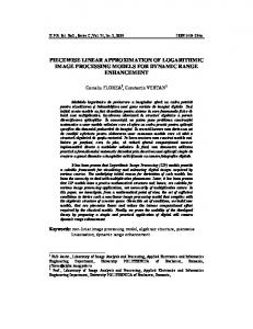
Piecewise Linear Image Coding Using Surface Triangulation and Geometric Compression Tianyu Lu, Zisheng Le and D. Y. Y. Yun Department of Electrical Engineering, University of Hawaii at Manoa Abstract The provably NP-hard problem of finding optimal piecewise linear approximation for images is extended from 1D curve fitting to 2D surface fitting by a dual-agent algorithm. The results not only yield a storage-efficient codec for range, or intensity, images but also a surface triangulation technique to generate succinct, accurate and visually pleasant 3D visualization model. Comparing with the traditional piecewise linear image coding (PLIC) algorithms, triangulation of a range image is more adaptive due to conformity of the shape, orientation and size of triangles with the image contents. The triangularization algorithm presented here differs from previous approaches in that it strives to minimize the total number of triangles (or vertices) needed to approximate the image surface while keeping the deviation of any intensity value to within a prescribed error tolerance. Unlike most methods of bottom-up triangularization, which could bog down before any mesh simplification even begins, this algorithm fits the surface in a top-down manner, avoiding the generation of most unnecessary triangles. When combined with an efficient 3D triangulation-encoding scheme, the algorithm achieves compact code length with guaranteed error bound, thus providing a more faithful representation of all image features. A variety of benchmark test images have been experimented and compared. Keywords: near-lossless image coding, piecewise linear image coding, surface modeling, mesh generation, surface triangulation, and geometric compression. 1. Introduction Real world applications continuously generate gigantic amount of data. To transmit and store such data, compression techniques are essential, particularly in the case of images. As Saupe [1] pointed out, in applications such as medical imagery, SAR satellite pictures and numerical weather simulation, due to the sensitivity of the data, there is a need for guaranteeing that the error of each component is within a certain tolerance. This is known as near-lossless coding or L∞-coding. One category of the image coding techniques ensuring such error bound is piecewise linear image coding (PLIC). Though Saupe achieved an elegant dynamic programming solution, his curve fitting based approach throws away the correlation among pixels due to the 2D-to-1D conversion. This research is motivated by the need to generalize PLIC for surface approximation. In this paper, as shown in Figure 1, the grayscale image is treated as a digitization of a xymonotone surface that represents the graph of a continuous bivariate function. In particular, the most commonly used range images in the field of computer vision are obtained by a range scanner from a fixed viewing direction and returned as an array of distance values. It often represents an orthogonal view of the boundary surface of a 3D object and thus referred to as 2½D data set. The problem addressed in this paper is formally defined as: Let ƒ(x,y) be a continuous bivariate function, and S be a set of points

uniformly sampled from ƒ in a rectangular domain W×H. A continuous PL function ϕ is called an ε-approximation of ƒ, for ε>0, if error e(p)=|ϕ(xp,yp)-zp|≤ε for every point p=(xp,yp,zp)∈S. In this paper, given S and ε, the PL surface approximation problem is to compute a PL function ϕ* in the form of a manifold triangular mesh that ε-approximates ƒ with the minimum number of triangles whose vertices form a subset S’ of S. Manifold triangular mesh is the de facto standard rendering model for 3D graphics and visualization. As depicted in Figure 1c, it consists of triangular faces pasted together along their edges. Computing such surface triangulation (i.e. manifold triangular mesh) is non-trivial. It has been proven to be NP-hard [2]. In this research, agent and resource planning techniques are applied to pursue a near optimal solution to this multi-objective optimization problem. Finally, a scheme “edgebreaker” is applied for encoding triangle connectivity together with a novel vertex prediction model and Huffman coding for encoding the vertex coordinates.

Figure 1. “Sombrero”, z=sin(r)/r, where r=(x2+y2)1/2

2. Related Work Block-based image coding can be thought of as surface approximation. The image plane is divided into non-overlapping blocks and an error measurement is usually exercised to evaluate the approximation accuracy of the block that approximates the intensity surface patch over it. The well-known JPEG and vector-quantization simply partition an image into fixed-size blocks and then seek for spatial redundancy in the blocks. Segmenting image into variable block sizes (VBS) is accomplished by quad-tree decomposition [3]. However, this imposes excessively rigid rules on the placement of blocks and thus causes ineffective segmentation of the image. Chen and Yun [4] discussed flexible placement of rectangular blocks. Nevertheless, it is difficult to have the agreement between the rigid rectilinear segment boundaries and image edges of arbitrary orientation or position. Wu [5] introduced a more flexible scheme which recursively bi-partitions an image by a horizontal, 45° diagonal, vertical, or 135° diagonal cut that minimizes the total meansquare error. Agarwal [2] used planar trapezoidal segment and presented a recursive trapezoidal partitioning scheme using dynamic programming with high-polynomial complexity. This certainly increases the segmentation flexibility comparing with the previous VBS methods. However, clearly it is still not a convincing solution due to its limitation on the orientations of the edges. Not to mention that such approximation does not form a connected sheet of surface that serves rendering purpose. Instead, this paper argues the superiority of surface triangulation. Triangles can be in arbitrary shape, orientation and size, thus, naturally adapt to the surface curvatures and fully explore the neighboring pixels correlations, resulting in more concise approximations. Surface approximation using polygonal models has been extensively utilized in the field of computer graphics. Many popular methods start from an over-sampled triangulation model such as those generated from volume data [6], laser scans [7] and satellite imagery

[8] and then aim at reducing the complexity of this large complex [9,10]. Overall, such two-stage approach is inherently memory-intensive. It generates a large number of triangles, many of which do not contribute relevant detail to the resulting model and end up being discarded at the simplification stage. It is desirable if the triangulation process can carry on both objectives − accuracy and conciseness in a single pass. In addition, the heuristic or energy-minimization based simplification schemes come with no performance guarantee, and generally do not have a quantitative quality measurement about the surface approximation they compute. These problems have begun to draw attentions recently. Cohen [11] computes a simplified approximation from a given fully detailed polygonal model, such that all points of the approximation are within a userspecified distance ε from the original model and vice versa. Weimer and Warren [12] guarantees similar error bound in constructing approximating triangulation of large terrain data. They adopt an iterative refinement approach where points with large error are inserted one by one. A Delaunay triangulation is maintained in the parameter plane. Such data-independent triangulation clearly ignores the image semantics, and therefore is far from optimal in terms of minimizing number of triangles. Agarwal [2] emphasized the importance of having quantitative measurement and used distance error bound. 3. Triangulation Generation Constrained Resource Planning (CRP) [14] is a decision process that focuses on the utilization of resources and the scheduling of related activities, in order to achieve goals while satisfying constraints. From the viewpoint of CRP, the triangulation process is to utilize the least amount of resources (triangles) to achieve the uniform error bound by a sequence of “split” and “merge” operations. The PL approximation problem has two somewhat conflicting objectives – maximizing model quality and minimizing model size. This research presents a dual-agent [13] system to attack this dual-objective optimization problem. Each agent specialized in optimizing one of the objectives works independently but coordinates with each other concurrently to strike the balance of the objectives. Starting with a rough initial triangulation, split-agent (perfectionist) adds points to refine the under-estimated regions to achieve better approximation quality, while merge-agent (economist) removes triangles at over-estimated regions to enforce model economy without incurring excessive error. The CRP engine helps them to determine the sequence of operations to reach convergence (thus achieve approximation quality) most efficiently (with the least resource). The cooperation and competition between agents is the driving force for the triangulation to converge to the original surface with the fewest possible triangles. This iterative refinement and relaxation process continues until the error at any point falls below the given tolerance ε and no more vertices can be taken out of the triangulation without incurring additional error points. The algorithm requires finding a coarse initial triangulation T0 covering all points of S. T0 can be as simple as only two triangles determined by the four corner points of the bounding box of S. Alternatively, a triangulation of a carefully chosen set of break points including the four corner points suffices [20]. 3.1. Split Algorithm

The goal of a split is to reduce model error and bring as many as possible points into error bound. The order to split triangles and the priority to pick split points surely make difference on the triangulation. Split agent always splits the triangle that has the largest number of error points. The split point is usually chosen to be the one that has the largest error. In case of ties, secondary criteria such as error point percentage, and total error are applied as tiebreakers. A B

A

D

A

D

D

F

F A

P

P

C D

B

B

C

C

B

E

E

C

Figure 2. Split, diagonal swapping and propagation

The split point P is connected with the three triangle vertices (A, B, C in figure 2b). To minimize the number of triangles while refining the approximation, the best triangulation configuration after each point insertion should be obtained. The optimality is that any quadrilateral formed by two neighboring triangles is triangulated using the diagonal that leads to less number of error points comparing with its alternative. This operation is called diagonal swapping. If both configurations result in the same amount of error points, the one that satisfies the Delaunay (MAX-MIN angle) condition is preferred. As shown in figure 2a, quadrilateral ABCD can be triangulated with diagonal AB or CD. In figure 2b, the quadrilateral formed by a new triangle (PAB) and its neighboring triangle (ADB) is checked to decide whether diagonal (AB) should be swapped. The two triangles resulted from this swap (ADP and BPD in 2c) will be checked with their neighbors recursively. Swap is valid only if the projection of the quadrilateral on the image plane is convex. This ensures that the orientation of the triangles will not reverse. It also means that, the swap originated at APF can only possibly propagate within the fan area (in 2b) formed by PA and PF. The propagation is indeed to draw points to become P’s direct neighbors. An important observation on the splitting process, thus, is that adding a new point to the triangulation only entails a local change of the triangulation while triangles far away remain intact. This limits the extent of change in the approximation and therefore will not increase the computational complexity. 3.2. Merge Algorithm The goal of a merge is to remove point to compact the model. However, it is subject to not increasing the total number of error points in its neighboring triangles. This usually occurs at flat region in the triangulation where large triangle can approximate the area sufficiently well. Therefore, the priority to merge vertices is the “flatness” of their neighborhood. As shown in figure 3a, the vertex-neighborhood of R is the set of triangles sharing R. We evaluate this “flatness” in terms of the maximum deviation of the normals of neighboring triangles from the surface normal nc at R. nc is estimated as an areaweighted average of the neighboring triangle normals. Merge agent always tries to remove vertex in the most flat neighborhood first. Again, secondary criteria such as total number of error points or total error are designed to break ties.

As depicted in figure 3, removal of a vertex introduces a “polygonal” hole. A triangulation for the polygon needs to be re-computed so that it is closest to the previous. A dynamic programming algorithm is formulated for constructing such optimal polygon triangulation. Let ƒ(vi,vj,vk) be a “closeness” measure of triangle (vi,vj,vk) to the surface patch it approximates. Let ƒ(T) be the overall approximation quality of a triangulation T, which is defined as the summation of the “closeness” measures of all the triangles it consists. As shown in figure 3c, the vertices of polygon P are numbered by v1, v2, …, vn, in counter-clockwise order around the perimeter. If vivj is a diagonal of P, P(i,j) denotes the polygon formed by points vi, vi+1, …,vj. Let F(i,j) be the minimum value of ƒ on a triangulation of P(i,j). If vivj is not a “valid” diagonal, define F(i,j)=+∞. A diagonal is valid if its projection is totally inside the polygon on the projection plane and noncollinear with any boundary edge. Obviously, we wish to compute F(1,n). Note that in any triangulation of P(i,j), vivj must be an edge of a triangle, say vivjvk, with i