Copyright © 2002 IFAC 15th Triennial World Congress, Barcelona, Spain
OPTIMAL PID TUNING WITH GENETIC ALGORITHMS FOR NON LINEAR PROCESS MODELS J.M. Herrero, X. Blasco, M. Martínez, J.V. Salcedo
1
Predictive Control and Heuristic Optimization Group Department of Systems Engineering and Control Universidad Politécnica de Valencia Camino de Vera 14, P.O. Box 22012 E-46071 Valencia, Spain Tel: +34-963877000 ext: 5713 . Fax: +34-963879579. E-mail:
[email protected] http://ctl-predictivo.upv.es
Abstract: This work presents a powerful and flexible alternative for tuning PID controllers using Genetic Algorithms. The potential of this technique is shown using non-linear process models and a reference trajectory. Flexibility is demonstrated by showing how to tune an optimal PID in various situations: model errors, noisy input, IAE minimization, and following a reference models, etc. These problems are solved by changing the minimization index. Copyright ©2002 IFAC. Keywords: Genetic Algorithms, Optimization, PID, Robust Control, Non-linear Control.
1. INTRODUCTION PID controllers are the most common controllers in industry, in fact, 95% of control loops use PID and the majority are PI. (Aström and Hägglund, 1995). Accordingly, there are many tuning techniques, and most are based on: (1) Empirical methods, such as Ziegler-Nichols methods. (Aström and Hägglund, 1995). (2) Analytical methods, for instance, the root locus based techniques. (Aström and Hägglund, 1995) (Blasco et al., 2000). (3) Methods based on optimization, such as Ciancone or Lopez methods (Marlin, 1995). These obtain PID parameters by optimising an IAE index and a linear model with the following structure. G(s) =
1
k p −θ s e τs + 1
This work has been partially financed by European FEDER funds, project 1FD97-0974-C02-02.
In all of these cases, PID tunings are obtained for an operation point where the model can be considered linear. This implies there is sub-optimal tuning when a process operates outside the validity zone of the model. This situation is common when the reference is not a set point but a trajectory (robot control, heating trajectories in furnaces, etc.). An alternative method to solve this problem is to obtain a model for different operational zones, tune a PID controller for each, and establish a mechanism for changing from one controller to another depending on the operation zone (gain planning). Another alternative is tuning a PID controller by taking into account all non-linearities and additional process characteristics. At this point appears the idea of using Genetic Algorithms (Herreros et al., 2000) (a global optimization technique) to obtain a PID tuning that meets all the requirements established in a minimization index by the designer.
• x1 , x2 : temperatures (in oC) involved in heating exchange (internal variables). • k1 , k2 : model parameters. Nominal parameters are k1 = 86 · 10−6 and k2 = 6.027 · 10−3.
2. GENETIC ALGORITHMS Genetic Algorithms (GA) (Goldberg, 1989), (Holland, 1975) are optimization techniques based on simulating the phenomena that takes place in the evolution of species and adapting it to an optimization problem. These techniques imply applying the laws of natural selection onto the population to achieve individuals that are better adjusted to their environment. The population is nothing more than a set of points in the search space. Each individual of the population represents a point in that space by means of his chromosome. The individual’s degree of adaptation is given by the objective function. Applying genetic operators to an initial population simulates the evolution mechanism of individuals. The most usual operators are as follows: • Selection: The main goal is selecting the chromosomes with the best qualities for integration in the next generation (these would depend on the cost function for each individual). • Crossover: By combining the chromosomes of two individuals, new chromosomes are generated and integrated into the population. • Mutation: Random variations of parts of the chromosome of an individual in the population generate new individuals. The variations of the Genetic Algorithms can be distinguished by the kind of codification used for the chromosomes and the genetic operators used.
Input Voltage (u)
Measured Resistance Temperature (y)
Regulated Power Supply
Resistance
Temperature Sensor
Resistance Temperature (ºC)
Inside Temperature Tin (ºC)
Fig. 1. Thermal Process Scheme. As usual, control tuning has to achieve different types of specification, such as: (1) Obtaining dynamic performances evaluated with: • minimization of a performances index such as IAE (integral of absolute value error). • Adjusting time specifications. (2) Obtaining robustness properties: • Model error robustness. • Input noise robustness. GA is simply a global and powerful optimization technique and, to use it in the tuning process, it is necessary translate all these types of specification to a cost function that the GA has to minimize. The advantage of a GA is that it is possible to solve very complicated cost functions and that allows the PID designer to establish any type of specification.
GA have demonstrated very good performances as global optimisers in many types of applications (Michalewicz, The following explains how to adjust the PI controller 1996), (Blasco et al., 1998) (Blasco, 1999). (two parameters, Kc and Ti ) 2 for different types of specification in order to control the thermal process. 3. OPTIMAL PID FOR A THERMAL PROCESS CONTROL A thermal process (figure 1) is used to illustrate the application of Genetic Algorithms to PID controller tuning. This process presents non-linearities, saturation model errors, and input noises. The state space representation is used and the parameters are obtained by identification using GA (?): x˙1 = k1 · u2 − k2 (x1 − Tin ) 1 x˙2 = (x − x2) 16.75 1 yˆ = x2 where: • y: ˆ resistance temperature in oC (Controlled variable). • u: voltage percentage at the control of the actuator (manipulated variable). • Tin : air temperature (in oC) in the resistance neighbourhood (Disturbance).
At the end of this section a summary table with the PI controllers, which has been designed for the IAE minimization, model error and input noise robustness, will be shown.
3.1 PI tuning for reference model In this case, the objective is to obtain a controlled variable following a time specification 3 . This type of specification can be represented as an ideal closed loop model - called the reference model. Now the tuning process has to minimize, over a simulation time (tsim ), differences between reference model output (ymr (t)) and the non-linear model controlled by the PI output (y(t)), see figure 2. This is represented as a cost function: 2
PI used is an ISA standard structure with anti-windup. PI(s) = kc (1 + 1/(Ti s)) 3 Restricción on: settling time t , overshoot δ , steady-state errors, e etc.
Trajectory Generator
yr
Non linear model of Thermal Process
PI
Output
y kc
2.15
2.1
Reference Model
MR Output
Optimizer
ymr
5
10
15
20 iterations
25
30
35
40
5
10
15
20 iterations
25
30
35
40
5
10
15
20 iterations
25
30
35
40
580
Ti
570
Fig. 2. Tuning structure for reference model.
560 550
tsim
J(Kc , Ti ) = ∑ |ymr (t) − y(t)|
66.8
(1) J(kc,Ti)
t=0
Reference models used in this examples, have been selected to achieve these specifications: • Settling time te (98%) = 100seconds • Overshoot δ = 0% • Steady-state error e p = 0
Fig. 3. Kc , Ti and J(Kc , Ti ) evolution for reference model optimization. 64
(2)
The optimization problem is two-dimensional (two parameter Kc , Ti ), there is no guarantee that it is a convex problem (non-linear model, saturation, PI antiwindup, etc.), and there is no computational restriction (off line optimization). Therefore, GAs offer a good alternative for solving the problem. GA characteristics are: • • • •
Real codification chromosome. Number of individual: 400. Ranking operator. Selection operator: Stochastic universal sampling. • Crossover operator: Intermediate recombination with a probability of 0.85. • Mutation operator: Random with a Gauss distribution (σ = 2%) and a probability of 0.05. o • Search space: Kc ∈ [0.1 . . . 20] %C and Ti ∈ [10 . . . 600]sec. The solution is: Kc = 2.14 , Ti = 559.97 , J(Kc , Ti ) = 66.24 Figure 3 shows Kc , Ti and J(Kc , Ti ) evolution during the optimization process. It shows optimization process convergence in the 20th iteration. The high number of individuals and the GA operator selected assure a good search space exploration, and that means the solution has a high degree of confidence. Figure 4 shows control results obtained with this solution and compared with the reference model.
63 Temperature(ºC)
1 C (25s + 1) %
66.4 66.2
62 61 60
Reference MR Output Output
59 58 57
0
50
100
150
200
250
300
350
200
250
300
350
Time(sec)
65 Manipulated Variable(%)
MR(s) =
66.6
60
55
50 0
50
100
150 Time(sec)
Fig. 4. PI closed loop control for reference model. (figure 5). That means, minimizing the following cost index: tsim
J(Kc , Ti ) = ∑ |yr (t) − y(t)|
(3)
t=0
Where yr (t) is the reference trajectory, y(t) is the model closed loop simulation with PI controller, and tsim is the simulation time. Trajectory Generator
yr PI
Non linear model of Thermal Process
Output
y
Optimizer Fig. 5. Tuning structure for IAE minimization.
3.2 PI tuning for IAE minimization The objective is adjusting PI parameters Kc and Ti to minimize the IAE index of closed loop response
The GA characteristics are the same as in the previous problem and the solution is: Kc = 9.18 , Ti = 179.13 , J(Kc , Ti ) = 533.07
Figure 7 shows optimization convergence behaviour is good. Figure 6 shows control result with the PI obtained.
j 1 2 3
66 reference output
Temperature(ºC)
64
k2 0.006027 0.006027 0.0075
PI parameters obtained are:
62 60
Kc = 10.68 , Ti = 136.84 , J(Kc , Ti ) = 1645.90
58 56 0
100
200
300
400
500 Time(sec)
600
700
800
900
0
100
200
300
400
500 Time(sec)
600
700
800
900
Figure 8 shows closed loop control results with the optimal PI obtained. The IAE obtained for the nominal process is 540.14 which is greater than the 533.07 obtained when it was only optimised for the nominal process. Figure 9 shows evolution during the optimization process.
100 80 60 40 20
66 0
reference output
64 Temperature(ºC)
Manipulated variable (%)
k1 0.000086 0.000110 0.000086
Fig. 6. PI closed loop control for IAE minimization.
62 60 58 56 0
100
200
300
400
500 Time(sec)
600
700
800
900
0
100
200
300
400
500 Time(sec)
600
700
800
900
kc
9.2
100
5
10
15
20 iterations
25
30
35
40
190
Ti
185 180
Manipulated variable (%)
9
80 60 40 20 0
175
5
10
15
20 iterations
25
30
35
40
J(kc,Ti)
533.3
Fig. 8. PI closed loop control for IAE minimization with model error robustness.
533.2 533.1 533
5
10
15
20 iterations
25
30
35
40
11.2 11 kc
Fig. 7. Kc , Ti and J(Kc , Ti ) evolution for IAE minimization.
10.8 10.6
5
10
15
20 iterations
25
30
35
40
5
10
15
20 iterations
25
30
35
40
5
10
15
20 iterations
25
30
35
40
145
3.3 PI tuning for model error robustness Ti
140 135 130 1646.6 1646.4 J(kc,Ti)
A method to increase robustness when there is model error, is by introducing in the cost index the minimization of the nominal process behaviour (IAE or reference model), y1 (t), and introducing the behaviour of several variations of the nominal process, y j (t) j 6= 1, (changing model parameters value). In this way, the cost index for IAE minimization follows a reference trajectory (yr (t)) and increasing robustness against model errors could be:
1646.2 1646 1645.8
Fig. 9. Kc , Ti and J(Kc , Ti ) evolution for IAE minimization with model error robustness.
n tsim
J(Kc , Ti ) =
∑ ∑ |yr (t) − y j (t)|
(4)
j=1 t=0
For instance, the PI of the thermal process is tuned while assuming three situations: firstly, ( j = 1) nominal parameters value, secondly, ( j = 2) an increase of 30% from nominal value in parameter k1 and thirdly, ( j = 3) an increase of 25% in k2 . Obviously, other situations can be added if necessary.
If model errors are present and the process parameters are: k1 = 0.000070 ; k2 = 0.0100 figure 10 compares nominal and robust PI closed loop simulations. Now the IAE obtained for the robust PI is 709.79, but the nominal PI IAE case obtained 866.49.
66 reference robust PI nominal PI
62
64 Temperature (ºC)
Temperature(ºC)
64
60 58
62 60 58
56 56 54
0
100
200
300
400
500 Time(sec)
600
700
800
900
80 60 40 20 0
100
200
300
400
500 Time(sec)
600
700
800
900
0
100
200
300
400
500 Time(sec)
600
700
800
900
100 Manipulated variable (%)
Manipulated variable (%)
100
0
0
100
200
300
400
500 Time(sec)
600
700
800
80 60 40 20 0
900
Fig. 10. Closed loop control with nominal and robust PI.
Fig. 12. Closed loop nominal process control with PI for noise robustness.
3.4 PI tuning for input noise
u
kc
11.3 11.25 11.2 11.15
Non-linear model Output of Thermal Process yn
10
15
20 Iterations
25
30
35
40
5
10
15
20 Iterations
25
30
35
40
5
10
15
20 Iterations
25
30
35
40
280 275 270 265 545.5
545
544.5
n
5
285
J(kc,Ti)
Cost index shows no changes in the IAE minimization and reference model after changing nominal behaviour (y(t)) for noisy behaviour (yn (t)), simply adding a noise (n(t)) with the same characteristics as the real one:
11.35
Ti
Another important source of problems in processes can be input noise. It can be possible to take this into account if the tuning optimization process simulates a noise of similar characteristics to that observed in the process.
Fig. 13. Kc , Ti and J(Kc , Ti ) evolution for IAE minimization with input noise.
Fig. 11. Structure with input noise. The cost index for a IAE minimization is:
66
tsimul
∑
|yr (t) − yn(t)|
(5)
t=0
For thermal processes, the noise is a random signal with a normal distribution of 10% amplitude.
reference nominal PI noise PI
64 Temperature (ºC)
J(Kc , Ti ) =
62 60 58 56 54
0
100
200
300
400
500 Time(sec)
600
700
800
900
0
100
200
300
400
500 Time(sec)
600
700
800
900
The obtained result is:
Figure 12 shows closed loop control results with the tuned PI. The IAE obtained for the nominal process without input noise is 542.45 which is greater than the 533.07 obtained when it was optimised only for nominal process. Figure 13 shows Kc , Ti and J(Kc , Ti ) evolution in the optimization process. With a normal distribution noise of 10% amplitude, the simulations are repeated for the nominal and noise PI. Obtained results are shown in figure 14. Now the IAE obtained for the noise PI is 544.79, but in the nominal PI case the IAE obtained is 600.67.
100 Manipulated variable (%)
Kc = 11.34 , Ti = 281.70 , J(Kc , Ti ) = 544.79
80 60 40 20 0
Fig. 14. Closed loop control with nominal and noise PI.
The following table shows the results obtained through the section.
PI Parameters kc , Ti 9.18,179.13 10.68,136.84 11.34,281.70
Nominal Process J(kc , Ti ) 533.07 540.14 542.45
Model Error J(kc , Ti ) 866.49 709.79 ...
Input Noise J(kc , Ti ) 600.67 ... 544.79
4. CONCLUSIONS This work shows how simple and powerful a GA application for controller tuning can be. Because the GA is a very good optimization technique, all control specifications that can be translated to a cost index can be applied. Application for different performance specifications (IAE minimization and restrictions in time domain) and robustness quality improvement (model errors and input noises) are shown. Everything applies to a nonlinear process. Only the application for a PID industrial controller is shown because it is one of the most important basic controllers. However, this technique can be applied to many linear and non-linear controllers. It is also possible to extend application to a multivariable control by simply adapting the cost index function. The only limitation is the computational cost of the optimization process - however, for off-line tuning this is not a major problem.
5. REFERENCES Aström, K.J. and T. Hägglund (1995). PID Controllers: Theory, Design, and Tuning. Instrument Society of America. Blasco, F.X. (1999). Model based predictive control using heuristic optimization techniques. Application to non-linear and multivariables proceses (In Spanish). PhD thesis. Universidad Politécnica de Valencia. Valencia. Blasco, F.X., M. Martínez, J. Senent and J. Sanchis (1998). Generalized predictive control using genetic algorithms (GAGPC). An application to control of non-linear process with model uncertainty. In: Methodology and tools in Knowledgebased systems (Springer, Ed.). Blasco, F.Xavier, M. Martínez, J. Senent and J. Sanchis (2000). Sistemas Automáticos. Editorial U.P.V. Goldberg, D.E. (1989). Genetic Algorithms in search, optimization and machine learning. AddisonWesley. Herreros, A., E. Baeyens and J.R. Perán (2000). Design of PID controllers using multiobjective genetic algorithms. In: Workshop on Digital control: Past, present and future of PID Control, PID’00 (Preprints, Ed.).
Holland, J.H. (1975). Adaptation in natural and artificial systems. Ann Arbor: The University of Michigan Press. Marlin, T. E. (1995). Process Control. Designing Processes and Control Systems for Dynamic Performance. Mc Graw-Hill. Michalewicz, Z. (1996). Genetic Algorithms + Data Structures = Evolution Programs. Springer.