Optimal Power Flow Using Firefly Algorithm with Consideration of ...

                   International Journal on Electrical Engineering and Informatics ‐ Volume 7, Number 1, March 2015 

Optimal Power Flow Using Firefly Algorithm with Consideration of FACTS Devices "UPFC" Ouafa Herbadji and Tarek Bouktir Dep. of Electrical Engineering, University of Sétif 1, Sétif, Algeria. [email protected] Abstract: This paper present solution of optimal power flow problem using a firefly algorithm (FA) with consideration of FACTS devices "UPFC". The objective is to minimize the total fuel cost of generation and also maintain an acceptable system performance in terms of limits on generator real power and reactive power outputs, bus voltages and power flow of transmission lines. In order to maximize the relief of congestion in power system, to reduce the total system real power loss and improves the loadability of the system we propose also the optimization of the placement of FACTS devices in the power system (UPFC). The proposed method is tested on IEEE 30-bus system and the Algerian electrical network. The result of this method is compared with those obtained by biogeography based optimization (BBO), genetic algorithm (GA), and artificial bee colony (ABC) algorithm. Keywords: Optimal power flow (OPF), Firefly algorithm (FA), Electrical network, FACTS, UPFC. 1. Introduction The problem of optimal power flow (OPF) has been one of the most widely studied subjects in the power system community [1]. He was first discussed by Carpentier in 1962[2]. The main goal of a generic OPF is to minimize the total thermal unit fuel cost, total emission, and total real power loss while up keeping the security of the system. In recent years, environmental constraint started to be considered as part of electric system planning. That is, minimization of pollution emission. The total emission can be reduced by minimizing the three major pollutants: nitrogen oxide (NOx), sulfur oxide (SOx), and carbon dioxide (CO2). In this study, Nitrogen-Oxide (NOx) emission is taken as the index from the viewpoint of environment conservation. So the total emission in the objective function will be considered in the OPF problem. In general, the total emission can be expressed as a non-linear function of power generation [3]. The unified power flow controller (UPFC) is an advanced member of the group of Flexible Alternating Current Transmission Systems (FACTS) with very attractive features [4]. This device can independently control many parameter, so it is the combination of the properties of a static synchronous compensator (STATCOM) and static synchronous series compensator (SSSC) [5]. It is able to control, simultaneously all the parameters affecting power flow in the transmission line: voltage, impedance, and phase angle [6]. Firefly algorithm (FA) is a meta-heuristic algorithm, developed by Xin-She Yang [7] for solving multimodal optimization problem. It based on the idealized behavior of the flashing characteristics of fireflies, including the light emission, light absorption and the mutual attraction. The objective of this paper is to develop an algorithm to simultaneously find the minimization of the total fuel cost of generation, maintain an acceptable system performance in terms of limits on generator real power, reactive power outputs, bus voltages and power flow of transmission lines and also to choose the best location of UPFC. This problem is solved using Firefly algorithm FA and Newton Raphson’s load flow method. It is tested on IEEE 30bus system and the Algerian electrical network. The result of this method is compared with

 Received: May 2nd, 2014. Accepted: February 25th, 2015 DOI: 10.15676/ijeei.2015.7.1.2

    those obtained by biogeography based optimization (BBO) [8], genetic algorithm (GA) [9], and artificial bee colony (ABC) algorithm [10]. This paper is organized as follows; The Problem formulation is presented in Section 2. In section 3, Modeling of UPFC is represented. The application of FA into optimal power flow is discussed in Section 4. In section 5, the case study including discussion is presented. Finally, conclusion is stated in Section6. 2. Problem formulation The standard OPF problem can be written in the following from: Subject to: 0 and 0

(1)

Where, is the objective function. is the equality constraints. is the inequality constraints. and is the vector of control variables, the control variable can be generated active power P , generation bus magnitudesV , and transformers tap T… etc. ,

, …

(2)

In this paper OPF is formulated as two objectives optimization problem as follows: A. Minimization of cost of generation The OPF problem can be expressed as minimizing the cost of production of the real power which is given by a quadratic function of generator power output P as [11, 12]. ∑

(3)

Where: is The fuel cost function. , , are the fuel cost coefficients. represent the corresponding generator (1,2,.....ng). is the generated active power at bus i. is number of generators including the slack bus. B. Minimization of NOx emission The amount of NOx emission is given as a function of generator output (in Ton/hr), that is the sum of quadratic and exponential functions. The objective function that minimizes the total emissions can be expressed as [13, 14]: ∑ Where results.

,

, ,

exp and

(4)

are the parameters estimated on the basis of unit emissions test

    C. The total objective function The pollution control can be obtained by assigning a cost factor to the pollution level expressed as: $/

(5)

Where is the emission control cost factor in $/Ton. 550.66 $/Ton. Fuel cost and emission are conflicting objective and can not be minimized simultaneously. However, the solutions may be obtained in which fuel cost an emission are combined in a single function with different weighting factor. This total objective function is described by [15]: $ ω 1 ω (6) 0 ω 1 (7) D. The equality and inequality constraints The OPF equality constraints g(x) reflects the physics of the power system, equality constraints are expressed in the following equation: ∑

0

(8)

is the total power demand of the plant. is the total power losses of the plant. The inequality constraints h(x) reflect the generators constraints and power system security limits. The inequality constraints on the problem variables considered include: • Upper and lower bounds on the active generations at generator buses Where;

P

P

P

(9)

• Upper and lower bounds on the reactive power generations at generator buses and reactive power injection at buses with VAR compensation Q

Q

Q

(10)

• Upper and lower bounds on the voltage magnitude at the all buses V

V

V

(11)

• Upper and lower bounds on the bus voltage phase angles θ

θ

θ

(12)

• Upper and lower transformer tap setting T limits are set as: T

T

T

(13)

3. Modeling of UPFC Unified Power Flow Controller (UPFC) is a multipurpose FACTS’s device which allows simultaneous control of active power flow, reactive power flow and the voltage magnitude at the UPFC terminals [16]. A simpler schematic representation of UPFC is shown in figure 1 with its equivalent circuit [17].

   

Figure 1. The UPFC equivalent circuit The UPFC equivalent circuit shown in Figure 1(b) consists of a shunt-connected voltage source, a series-connected voltage source, and an active power constraint equation, which links the two voltage sources. The two voltage sources are connected to the AC system through inductive reactance representing the VSC transformers. The UPFC voltage sources are [18]: (14) (15) and are the controllable magnitude and phase angle of the voltage source Where: representing the shunt converter respectively (equation (18),(19)). 0

2

(16) (17)

and are the controllable magnitude and phase angle of the voltage source representing the series converter respectively (equation (20),(21)). 0

2

The équation of the active power and reactive power at bus k and m are: cos sin cos sin cos sin cos sin cos sin cos sin cos sin cos sin

(18) (19)

(20) (21) (22)

    cos cos

sin

(23) sin

The active and the reactive power of the series converter : cos sin cos sin cos sin cos sin The active and the reactive power of the shunt converter : cos sin sin cos

(24) (25)

(26) (27)

4. Firefly algorithm for optimal power flow Firefly algorithm (FA) is a meta-heuristic algorithm, developed by Xin-She Yang [7] for solving multimodal optimization problem. It based on the idealized behavior of the flashing characteristics of fireflies, including the light emission, light absorption and the mutual attraction. For simplicity in describing our new Firefly Algorithm (FA), we now use the following three idealized rules [19-21]: 1. All fireflies are unisex so that one firefly will be attracted to other fireflies regardless of their sex. 2. Attractiveness is proportional to their brightness, thus for any two flashing fireflies, the less brighter one will move towards the brighter one. The attractiveness is proportional to the brightness and they both decrease as their distance increases. If there is no brighter one than a particular firefly, it will move randomly. 3. The brightness of a firefly is affected or determined by the landscape of the objective function. For a maximization problem, the brightness can simply be proportional to the value of the objective function. Other forms of brightness can be defined in a similar way to the fitness function in genetic algorithms. Based on these three rules, the basic steps of the firefly algorithm (FA) can be summarized as the pseudo code shown in Figure 2. Firefly Algorithm Objective function f(x), x = ( , ..., )T (i = 1, 2... n) Generate initial population of fireflies Light intensity Ii at xi is determined by f( ) Define light absorption coefficient while (t Ii), Move firefly i towards j in d-dimension; end if Attractiveness varies with distance r via exp[−r] Evaluate new solutions and update light intensity end for j end for i Rank the fireflies and find the current best end while Postprocess results and visualization Figure 2. Pseudo code of the firefly algorithm (FA)

    In the firefly algorithm, there are two important issues: the variation of light intensity I and formulation of the attractiveness β. The brightness of a firefly at a particular location x can be chosen as: (28) The light intensity I vary with the distance r. That is: (29)

Start

Initialize location of fireflies Iteration =1

Insert variable x into load flow data

Objective function evaluation

Ranking fireflies by their light intensity/objective

No Iteration   maximum

Find the current best solution Move all fireflies to the better locations

Yes Results

End

Figure 3. Optimal power flow using FA Where the original is light intensity and γ is the absorption coefficient. As a firefly’s attractiveness is proportional to the light intensity seen by adjacent fireflies, we can now define the attractiveness of a firefly by: 1

(30)

Where, β is the attractiveness at r =0, m is the number of the fireflies. The movement of a firefly i is attracted to another more attractive firefly j is determined by the equation: (31)

    With ∑

,

,

²

(32)

Where, r is the distance between two fireflies i and j at and , respectively, α is the size of the random step. The process of incorporating the firefly algorithm FA into optimal power flow is summarized in Figure 3 Where each firefly represents the values of the active power generated [22]. 5. Application study The OPF with FACTS device using Firefly algorithm (FA) approach has been developed and implemented by the use of Matlab 9. The applicability and validity of this method (FA) have been tested on IEEE 30-bus system and Algerian network (59-bus). To demonstrate the effectiveness of the proposed approach two cases to be discussed: Case 1: represent the solution of optimal power flow without FACTS device installed. Case 2: One UPFC device is installed. A. Application on the IEEE 30-bus system The IEEE 30-bus system consist of 6 generators (n°:1, 2, 5, 8, 11 and 13), 41 transmission lines and 4 transformers (Figure 4).

Figure 4. Structure of the tested IEEE 30 Bus System The active power generating limits and the unit costs of all generators of the IEEE 30-bus test system are presented in Table 1 [15], and the emission coefficients of generators are presented in Table 2 [23]. The total active load in the system was 283.4 MW, and the emission control cost factor for this system was taken as 550.66 $/Ton [24]. The voltage of generator buses and load buses are: ≤ 1.10 pu. The upper and lower bounds on the bus voltage phase angles are set 0.90 ≤ between -14 °& 0° and upper and lower transformer tap setting T limits are set between 0.95 & 1.1 pu.

    Table 1. Power generation limits and cost coefficients for IEEE 30-bus system Pgi Pgi(min) Pgi(max) Ai Bi .10 −2 Ci .10 −4 (MW) (MW) (MW) ($/MWh) ($/MW2h) ($/h) Pg1 50 200 0.00 200 37.5 Pg2 20 80 0.00 175 175.0 Pg5 15 50 0.00 100 625.0 Pg8 10 35 0.00 325 83.0 Pg11 10 30 0.00 300 250.0 Pg13 12 40 0.00 300 250.0 Table 2. Emission coefficients for IEEE 30-bus system bus

a.10-2 (Ton/h)

b.10-4 (Ton/ MWh)

c.10-6 (Ton/ MW²h)

d.10-4 (Ton/ MWh)

e.10-2 (Ton/MWh)

1 2 5 8 11 13

4.091 2.543 4.258 5.326 4.258 6.131

-5.554 -6.047 -5.094 -3.550 -5.094 -5.555

6.490 5.638 4.586 3.380 4.586 5.151

2.00 5.00 0.01 20.00 0.01 10.00

2.857 3.333 8.000 2.000 8.000 6.667

Table 3. The optimum generations for minimum total cost obtained by FA-OPF Variables ω =1 ω =0.5 ω =0 P1 (MW) 177.1034 129.6699 68.0558 P2 (MW) 48.8809 56.9540 70.9006 P5 (MW) 21.3295 25.4238 50.0000 P8 (MW) 20.8003 35.0000 35.0000 P11 (MW) 12.2012 23.1468 30.0000 P13 (MW) 12.0000 19.2363 32.8166 V1 (p.u) 1.0900 1.0900 1.0900 V2 (p.u) 1.0900 1.0818 1.0838 V5 (p.u) 1.0900 1.0585 1.0634 V8 (p.u) 1.0800 1.0706 1.0700 V11 (p.u) 1.0900 1.0900 1.0616 V13 (p.u) 1.0900 1.0900 1.0900 T6-9 (p.u) 0.9588 1.1000 1.0861 T6-10 (p.u) 1.0817 1.0975 1.1000 T4-12 (p.u) 1.0874 1.0048 1.1000 T28-27 (p.u) 1.1000 1.1000 1.0997 Power losses (MW) 8.9153 6.0308 3.3730 Generation cost ($/h) 800.0811 818.4117 933.6162 Emission (ton/h) 0.3684 0.2698 0.2174 Total cost ($/h) 1002.9442 966.9797 1053.3296

    The FA properties are set as follow: • Number of fireflies: 50. • Number of Iterations: 200. • Alpha (scaling parameter): 0.5 • Minimum value of betta (attractiveness): 0.2 • absorption coefficient: 1 Case 1: in this case the OPF is running without using the UPFC device and the vector of control variables include the generated active powers, magnitude voltages of generators and transformer tap settings. ,

,

,

,

,

,

,

,

,

,

,

,

,

,

]

(33)

The results including the generation cost, the emission level, total cost, generated active power, magnitude voltage, power losses and transformer tap settings are shown in Table 3. This table represent the optimum generations for minimum total cost in three cases: ω = 1: Minimum generation cost without using into account the emission level as the objective function. ω = 0.5: Equal influence of generation cost and pollution control in the objective function. ω = 0: A total minimum emission is taken as the objective of main concern. Table 4. Comparison with FA-OPF, BBO-OPF, GA-OPF and BBO-OPF

P1 P2 P5 P8 P11 P13

Variables

FA-OPF

BBO-OPF

GA-OPF

ABC-OPF

(MW) (MW) (MW) (MW) (MW) (MW)

176.7311 48.8454 21.4931 21.6923 12.1535 12.0000

171.9231 8.8394 1.4391 1.7629 2.1831 6.5588

176.7307 48.8488 21.4941 21.6881 12.1530 12.0009

180.5218 48.7845 21.2598 18.6469 11.8145 12.1011

Power losses (MW)

9.5155

9.3064

9.5156

9.7286

Generation cost ($/h)

802.3646

802.717

802.3647

802.1649

The active powers of the 6 generators as shown in this table are all in their allowable limits. We can observe that the total cost of generation and pollution control is the highest at the minimum emission level (ω=0) with the lowest real power loss (3.3730MW). As seen by the optimal results shown in the table 3, there is a trade-off between the fuel cost minimum and emission level minimum. The difference in generation cost between these two cases (800.0811$/hr compared to 933.6162$/hr), in real power loss (8.9153MW compared to 3.3730MW) and in emission level (0.3684Ton/hr compared to 0.2174 Ton/hr) clearly shows this trade-off. To decrease the generation cost, one has to sacrifice some of environmental constraint. The minimum total cost is at ω =0.5 of the order of 966.9797$/h. •

Comparison with FA-OPF, BBO-OPF, GA-OPF and BBO-OPF

    The comparisons of the results obtained by the proposed approach FA with those found by the biogeography based optimization BBO [8], genetic algorithm GA [9] and artificial bee colony ABC algorithm [10] are reported in the Table 4. This table gives the optimum generations for minimum total cost for ω =1 and the vector of control variables include only the generated active powers. The comparisons of the results between FA-OPF, BBO-OPF, GA-OPF and ABC-OPF show that the firefly algorithm gives acceptable solution. The FA gives very near results of fuel cost (802.3646$/hr) compared with the results obtained with those methods (802.717$/hr, 802.3647$/hr & 802.1649$/hr) and in the active power loss also. Case 2: in this case the OPF is running with using the UPFC device and the vector of control variables include only the generated active powers. The objective is to minimize the total fuel cost of generation, the power losses and the voltage deviations, we propose also the optimization of the placement of UPFC device in the power system. Table 5. Parameters of UPFC Xcr (pu) Xvr(pu) Qmax (MVar) Qmin (MVar) UPFC 0.45 0.3 35 -35 The total generation, active power, reactive power, total losses and optimal location of UPFC are shown in table 6. Table 6. Comparison of results obtained by FA-OPF with-without UPFC With Min Without UPFC UPFC Pg1 (MW) 50 176.7311 177.5808 Pg2 (MW) 20 48.8454 48.8800 Pg5 (MW) 15 21.4931 21.3200 Pg8 (MW) 10 21.6923 20.8000 Pg11 (MW) 10 12.1535 12.2000 Pg13 (MW) 12 12.0000 12.0000 Qg1 (MVar) -20 -4.3000 -4.7000 Qg2 (MVar) -20 25.8000 24.3000 Qg5 (MVar) -15 25.5000 24.9000 Qg8 (MVar) -15 13.9000 10.0000 Qg11 (MVar) -10 28.8000 26.6000 Qg13 (MVar) -15 31.8000 28.7000 Generation cost ($/h) 802.3646 800.0336 Active power losses 9.5155 9.3808 (MW) - 4.8 -5.9 Reactive Power losses (MVar) Optimal location of Ligne 33 UPFC (24-25) Q24=10.6 MVar

Max 200 80 50 35 30 40 200 100 80 60 50 60 -

The objective function is described by: ∑ ∑ With: nb is number of branches on the network.

∑

²]

(36)

    JB is number of buses. is the reference value of the bus voltage magnitude,: , are called the penalty factors.

1.0

.

The control parameters of UPFC are showed in Table 5.

1.1 1.08

Withou UPFC UPFC (bus 24) UPFC (bus 25)

1.06

V (pu)

1.04 1.02 1 0.98 0.96 0.94

0

5

10

15 Buses

20

25

30

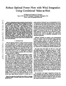
Figure 5. Voltage profile of all buses for IEE 30-bus system with &without UPFC The proposed approach with optimal installation of UPFC at line 33 (between buses 24 & 25) gives better results than without UPFC installation. For example with installation of UPFC, the fuel cost is 800.0336$/h, active power losses 9.3808MW and the reactive power losses -5.9 MVar which are better compared with the results found at the base case (without UPFC) (802.3646$/h, 9.5155MW and - 4.8 MVar). The FA method proposes other location of UPFC in critical lines; 16, 17, 18, 19, 22, 25, 26, 27, 28, 29, 30, 32, 39. We can observe also that the active powers and the reactive powers of the 6 generators as shown in the table 5 are all in their allowable limits. Figure 5 shows the voltage magnitudes profiles, it is clearly identified that all voltage magnitudes profiles are within the constraints limits and it was optimize after UPFC installation. B. Application on the Algerian network The FA-OPF has been also tested on the Algerian network. It consists of 59 buses, 83 branches and 10 generators. The slack bus is the bus N° 4. The generator of the bus 13 is not in service. (Figure 6).

   

Figure 6. Topology of the Algerian production and transmission network before 1997 (Sonelgaz). The active power generating limits and the unit costs of all generators of the Algerian network are presented in Table 7, and the emission coefficients of generators are presented in Table 8. The total active load in the system was 684.10 MW. Table 7. Power generation limits and cost coefficients for Algerian network Pmin

Pmax

Qmin

Qmax

A

B

C

MW

MW

Mvar

Mvar

$/h

$/MWh

$/MW2h

8 10 30 20 15 10 10 15 18 30

72 70 510 400 150 100 100 140 175 450

-10 -35 -35 -60 -35 -20 -20 -35 -35 -100

15 45 55 90 48 35 35 45 55 160

0 0 0 0 0 0 0 0 0 0

1.50 2.50 1.50 1.50 2.50 2.50 2.00 2.00 2.00 1.50

0.0085 0.0170 0.0085 0.0085 0.0170 0.0170 0.0030 0.0030 0.0030 0.0085

Bus 1 2 3 4 13 27 37 41 42 53

    bus 1 2 3 4 13 27 37 41 42 53

a.10-2 Ton/h 4.091 2.543 4.258 5.326 4.258 6.131 4.091 2.543 4.258 5.326

Table 8. Emission coefficients for Algerian network b.10-4 c.10-6 d Ton/MWh Ton/MW²h Ton/MWh -5.554 6.490 2.00 e-4 -6.047 5.638 5.00 e-4 -5.094 4.586 1.00 e -6 -3.550 3.380 2.00 e -3 -5.094 4.586 1.00 e -6 -5.555 5.151 1.00 e -5 -5.554 6.490 2.00 e -4 -6.047 5.638 5.00 e -4 -5.094 4.586 1.00 e -6 -3.550 3.380 2.00 e -3

e.10-2 Ton/MWh 2.857 3.333 8.000 2.000 8.000 6.667 2.857 3.333 8.000 2.000

Case1: FA-OPF without UPFC installation The table 9 gives the optimum generations for minimum total cost in three cases (total minimum generation cost ω=1, total minimum emission ω=0 and an equal influence of generation cost and pollution control in the objective function) Table 9. The optimum generations for minimum total cost obtained by FA-OPF for the Algerian network ω =1 ω =0.5 ω =0 Pg1 (MW) 60.3536 62.9017 70.0891 Pg2 (MW) 27.5474 43.1420 56.0679 Pg3 (MW) 102.8548 99.8792 85.2725 Pg4 (MW) 113.8841 108.4669 88.0140 Pg27 (MW) 24.9015 41.8344 91.5826 Pg37 (MW) 50.4757 50.3362 52.2015 Pg41 (MW) 97.0015 96.0575 91.6294 Pg42 (MW) 132.4250 110.7141 90.5276 Pg53 (MW) 104.7032 101.5773 86.6985 Vg1 (pu) 1.0314 1.0000 1.0114 Vg2 (pu) 1.0456 1.0826 1.0372 Vg3 (pu) 1.0345 1.0796 1.0046 Vg4 (pu) 1.0388 1.0673 1.0023 Vg27 (pu) 1.0382 1.0661 1.0014 Vg37 (pu) 1.0445 0.9976 0.9971 Vg41 (pu) 1.0671 0.9908 0.9874 Vg42 (pu) 1.0631 1.0047 1.0035 Vg53 (pu) 1.0241 1.0353 1.0213 Generation cost ($/h) 1699.9 1725.5 1820.2 Emission (ton/h) 0.4841 0.4455 0.4030 Power losses (MW) 30.0468 30.8094 27.9831 Total cost ($/h) 1699.9 1970.8190 2042.11 Time (s) 123.2973 100.5449 174.3222 The active powers generated as shown in table 9 are all in their allowable limits, the voltages magnitude also are within the constraint limit .We can observe also that the minimum total cost is at ω =1 of the order of 1699.9 $/h

    The comparisons of the results obtained by the proposed approach FA with genetic algorithm [9] are reported in the Table 10. This table gives the optimum generations for minimum total cost for ω =1 and the vector of control variables include only the generated active powers Table 10. Comparison with FA-OPF and GA-OPF FA-OPF Pg1 (MW) 51.5427 Pg2 (MW) 37.7899 Pg3 (MW) 100.3145 Pg4 (MW) 111.0000 Pg27 (MW) 28.7414 Pg37 (MW) 49.6008 Pg41 (MW) 105.6506 Pg42 (MW) 129.2478 Pg53 (MW) 100.1077 Generation cost ($/h) 1706.8000 Power losses (MW) 29.8000

GA-OPF 45,7786 40,6655 104,4367 110.0000 23,8188 51,4785 96,2285 123,4861 117,7484 1708.9 29.541

Table 11. Comparison of results obtained by FA-OPF with-without UPFC for the Algerian network Min Without With Max UPFC UPFC Pg1 (MW) 8 51.5427 51.5000 72 Pg2 (MW) 10 37.7899 37.8000 70 Pg3 (MW) 30 100.3145 100.3000 510 Pg4 (MW) 20 111.0000 109.6000 400 Pg27(MW) 10 28.7414 28.7000 100 Pg37(MW) 10 49.6008 49.6000 100 Pg41(MW) 15 105.6506 105.7000 140 Pg42(MW) 18 129.2478 129.2000 175 Pg53(MW) 30 100.1077 100.1000 450 Qg1(MVar) -10 -03.0000 -0.3000 15 Qg2(MVar) -35 17.4000 15.3000 45 Qg3(MVar) -35 46.0000 45.0000 55 Qg4(MVar) -60 46.8000 47.3000 90 Qg27(MVar) -20 35.0000 35.0000 35 Qg37(MVar) -20 17.6000 17.6000 35 Qg41(MVar) -35 45.0000 45.0000 45 Qg42(MVar) -35 19.0000 19.1000 55 Qg53(MVar) -100 01.0000 -12.4000 160 Generation cost ($/h) 1706.8000 1702.1000 Active power losses 29.8000 28.4000 (MW) Reactive Power losses -19.7000 -21.3000 (MVar) Line 66 Optimal location of (36-43) UPFC Qg36=14.3 MVar

    The results obtained with proposed approach FA-OPF are better than those obtained by GA-OPF (1706.8000 $/h & 29.8000 MW) compared to (1708.9$/h & 29.541 MW). Case2: FA-OPF with UPFC installation In this case the OPF is running with using the UPFC device and the vector of control variables include only the generated active powers. From the comparison table 11, the proposed OPF method with UPFC loss is lesser than proposed OPF method without UPFC. The proposed OPF method with UPFC loss is reduced as 28.4000MW when the optimal location of UPFC is at line 66 between buses 36 & 43. Also, the fuel cost is reduced after installation of UPFC (1702.1000 $/h) compared to (1702.1000 $/h). Hence, the solution of optimal power flow problem using a firefly algorithm (FA) with UPFC is better for analyzing power flow of electric power system. The FA-OPF method proposes other location of UPFC in critical lines: 20, 21, 22, 24, 25, 34, 38, 39, 57, 63, 66, 67, 73, 75, and 76. 1.15

without UPFC

With UPFC

Min

Max

1.1

V (pu)

1.05 1 0.95 0.9 X: 36 Y: 0.825

0.85 0

10

20

30 Buses

40

50

Figure 7. Voltage profile of all buses for Algerian network with & without UPFC Figure 7 shows the voltage profile with and without UPFC. It is clearly identified that all voltage magnitude profiles are within the constraint limit. 7. Conclusion In this paper, a new swarm based Firefly Algorithm has been presented to solve the optimal power flow problem with consideration of FACTS devices "UPFC". The FA-OPF has been successfully implemented to solve optimal power flow problem for minimization of the total cost of the generation, the cost of pollution level control and the active power loss. The proposed method is tested on IEEE 30-bus system and the Algerian electrical network. Simulation results show that the solution of optimal power flow problem using a firefly algorithm (FA) with installation UPFC in right location is better for analyzing power flow of electric power system. 8. References [1] Hongye Wang, Carlos E. Murillo-Sanchez, Ray D. Zimmerman and Robert J. Thomas, "On Computational Issues of Market-Based Optimal Power Flow", IEEE Transactions on Power Systems, Vol. 22, No. 3, pp: 1185-1193, Aug 2007. [2] J. Carpentier, "Contribution a l’étude du dispatching économique", Bulletin de la Société Française des Electriciens, vol. 3, pp. 431–447, Aug. 1962.

    [3] Ruey-Hsun Liang, Sheng-Ren Tsai, Yie-Tone Chen, Wan-Tsun Tseng, "Optimal power flow by a fuzzy based hybrid particle swarm optimization approach", Electric Power Systems Research, Vol.81, 1466–1474, 2011. [4] D. Murali, M. Rajaram, "Active and Reactive Power Flow Control using FACTS Devices", International Journal of Computer Applications (0975 – 8887) Volume 9– No.8, November 2010. [5] S. Muthukrishnan and A. Nirmal Kumar, " Comparison of Simulation and Experimental Results of UPFC used for Power Quality Improvement", International Journal of Computer and Electrical Engineering, Vol. 2, No. 3, 1793-8163, June, 2010. [6] L. Gyugyi, C.D. Schauder, S.I. Williams, T.R. Reitman, D.R. Torgerson, and A. Edris, 1995, "The Unified Power Flow Controller: A new approach to power transmission control", IEEE Trans. on Power Delivery, 10(2), pp. 1085-1097. [7] X.-S. Yang, "Firefly algorithms for multimodal optimization," Stochastic Algorithms: Foundation and Applications SAGA 2009, vol. 5792, pp. 169-178, 2009. [8] O. Herbadji, L. Slimani and T. Bouktir, "Biogeography Based Optimization Approach for Solving Optimal Power Flow Problem", International Journal of Hybrid Information Technology Vol.6, No.5, pp.183-196, 2013. [9] T. Bouktir, L. Slimani, M. Belkacemi, "A Genetic Algorithm for Solving the Optimal Power Flow Problem", Leonardo Journal of Sciences, 2004. [10] L. Slimani and T. Bouktir, "Optimal Power Flow with Emission Controlled using Artificial Bee Colony Algorithm", 12th International conference on Sciences and Techniques of Automatic control & computer engineering, Sousse, Tunisia, 2011. [11] A. J. Wood and B.F. Wollenberg, "Power Generation, Operation and Control" , 2nd Edition, John Wiley, 1996. [12] Glenn W. Stagg, Ahmed H. El Abiad, "Computer methods in power systems analysis", McGraw-Hill, 1981. [13] L. Slimani and T. Bouktir, "Economic Power Dispatch of Power System with Pollution Control using Multiobjective Ant Colony Optimization", International Journal of Computational Intelligence Research., ISSN 0973-1873 Vol.3, No.2, 145-153, 2007. [14] B. Mahdad, T. Bouktir and K. Srairi, "OPF with Environmental Constraints with Multi Shunt Dynamic Controllers using Decomposed Parallel GA: Application to the Algerian Network", Journal of Electrical Engineering & Technology, Vol. 4, No.1, 55~65, 2009. [15] T. Bouktir and M. Belkacemi, "Object-Oriented Optimal Power Flow", Electric Power Components and systems, Vol. 31, (6) 525-534, 2003. [16] Behzad Minooie and Mostafa Sedighizadeh, “Optimal Site and Parameters Setting of UPFC Based on Hybrid Genetic Algorithm for Enhancing Loadability”, Technical Journal of Engineering and Applied Sciences, ISSN 2051-0853 , 2013. [17] E. Acha, V. G. Agelidis, O. Anaya-Lara and T. j. Miller, "Power electronic control in electrical systems", 1st edition, Newnes, 2002. [18] Enrique Acha, Claudio R. Fuerte-Esquivel, Hugo Ambriz-Pérez and César AngelesCamacho, " FACTS, Modelling and simulation in power networks" , 2004. [19] S. Lukasik and S. Zak, "Firefly algorithm for con-tinuous constrained optimization tasks", in Proceedings of the International Conference on Computer and Computational Intelligence (ICCCI ’09), N. T. Nguyen, R. Kowalczyk, and S.-M. Chen, Eds., vol. 5796 of LNAI, pp. 97–106, Springer, Wroclaw, Poland, October 2009. [20] X. S. Yang, "Firefly algorithm, Levy flights and global optimization", in Research and Development in Intelligent Systems XXVI, pp. 209–218, Springer, London, UK, 2010. [21] X. S. Yang, "Firefly algorithm, stochastic test functions and design optimization", International Journal of Bio-Inspired Computation, vol. 2, no. 2, pp. 78–84, 2010. [22] O. Herbadji, N. Ketfi, L. Slimani, T. Bouktir, " Optimal power flow with emission controlled using firefly algorithm", 5th International Conference on Modeling, Simulation and Applied Optimization, ICMSAO 2013, art. no. 6552559, 2013.

    [23] T. Bouktir, B R. Lab bdani and L. Slimani, "Economic Power Disspatch of Poweer System withh Polluution Control using u Multiobjjective Particlee Swarm Optim mization", Jourrnal of Pure & Applied Sciences, Vol.4, V No. 2 577-77, 2007. [24] L. Slimani, S T. Bouktir, "Optimal Power Flow using Artificial A Bee Colony withh Incoorporation of FACTS F Devicces: a Case Study", Internaational Review w of Electricall Engineering, Vol. 6 N. 7, Papers Part B, Decem mber 2011. Ouafa Herbadji H was born b in Setif, Algeria A in 19887. She receiveed the engineeering degree inn electrical engineering frrom Sétif 1 Unniversity (Algeeria) in 2010 annd the Magisteer degree from m Universityy of Setif 1 in 2014. Now shhe is conductinng his doctoral research at thee University off Setif 1, Algeria. A Her areea of interest is i the applicatiion of the metaa-heuristic metthods in powerr systems analysis. a Tarek k BOUKTIR was born in Ras El-Oued, Algeria in 19971. He is thee Editorr-In-Chief of Journal J of Elecctrical Systemss (Algeria), the Co-Editor off Journ nal of Automaation & System ms Engineerinng (Algeria). He H is with thee Deparrtment of Elecctrical Engineeering in Setif 1 University, ALGERIA. A Hee curren ntly serves as a member of thhe Board of thee University off sétif 1.