Optimal Power Flow with Emission Controlled using Firefly Algorithm Ouafa Herbadji1, Ketfi Nadhir2 1
Dep. of Electrical Eng., University of Sétif 1, Algeria. Dep. of Electrical Eng., University of Batna, Algeria.
[email protected]
2
Abstract—This paper presents the use of a meta-heuristic nature-inspired algorithm, called firefly algorithm for the solution of the optimal power flow problem. The objective is to minimize the total fuel cost of generation and environmental pollution caused by fossil based thermal generating units and also maintain an acceptable system performance in terms of limits on generator real and reactive power outputs, bus voltages, shunt capacitors/reactors and power flow of transmission lines. In this work the standard IEEE 30-bus test system with six generating units has been used to test the effectiveness of the proposed method. Satisfactory results obtained from the proposed method were compared to those obtained by genetic algorithm (GA) and particle Swarm methods (PSO). Keywords—Optimal Power Flow; Power Systems; Pollution Control; Firefly algorithm (FA).
I.
INTRODUCTION
The optimal power flow (OPF) problem has been one of the most widely studied subjects in the power system community [1]. The goal of optimal power flow (OPF) is to find an optimum combination of real power generation levels, voltage magnitudes, and tap positions for the transformer load tap changer (LTC) to minimize the total thermal unit fuel cost, total emission, and total real power loss while satisfying physical and technical constraints on the network. Nitrogen oxides (NOx) emissions, produced in a thermal power plant, have harmful effects on both the environment and human health. Strict legislations have been introduced recently in many industrial countries to modify their operational strategies to restrict such pollutant emissions [2]. The NOX emissions will be considered in the OPF problem for environmental protection. So the total emission in the objective function will be considered in the OPF problem. In general, the total emission can be expressed as a non-linear function of power generation [3]. One of the most recent meta-heuristic algorithms, the Firefly algorithm (FA) for solving multimodal optimization problem by Xin-She Yang [4], it’s based on the firefly bugs behavior, including the light emission, light absorption and the mutual attraction. In this paper, a new swarm intelligence approach that utilizes Firefly Algorithm (FA) is proposed to solve the
978-1-4673-5814-9/13/$31.00 ©2013 IEEE
3
Linda Slimani , Tarek Bouktir
3
3
Dep. of Electrical Engineering, University of Sétif 1 Sétif, Algeria.
[email protected] optimal power flow problem using as objective function the minimization of the fuel cost and polluted gas emission. To verify the approach and for comparison purposes, we perform simulation on IEEE30 bus system with six generating. The obtained results are compared to the genetic algorithm (GA) and Particles Swarm Optimization (PSO) methods [5]. This paper is organized as follows; The Problem formulation is presented in Section 2. The concept of FA is presented in Section 3, The application of FA into optimal power flow is discussed in Section 4. In section 5, the case study including discussion is presented. Finally, conclusion is stated in Section6. II. PROBLEM FORMULATION The standard OPF problem can be written in the following from: Min F x (2.1) Subject to: g x 0 (2.2) And h x 0 (2.3) Where, F x is the objective function. g x is the equality constraints. h x is the inequality constraints and And x is the vector of control variables, the control variable can be generated active and reactive power, generation bus magnitudes, and transformers tap etc. x P ,P ,P …P ,V ,V …V ,… Where, ng is the number of generators buses.
(2.4)
A. The objective function In this paper OPF is formulated as two objectives optimization problem as follows: •
Minimization of cost of generation
The most commonly used objective in the OPF problem formulation is the minimization of the total cost of real power generation. The fuel cost curve is assumed to be approximated by a quadratic function of generator power output P as [6, 7].
F
∑
∑
F
A
BP
CP
$/h
(2.5)
Where: A ,B , C are the fuel cost coefficients. i represents the corresponding generator (1,2,.....ng). P is the generated active power at bus i. ng is number of generators including the slack bus. •
∑
The emission control cost results from the requirement for power utilities to reduce their pollutant levels below the annual emission allowances assigned for the affected fossil units. The total emission can be reduced by minimizing the three major pollutants: oxides of nitrogen, oxides of sulphur and carbon dioxide. The objective function that minimizes the total emissions can be expressed in a linear equation as the sum of all the three pollutants resulting from generator real power [8]. The amount of NOx emission is given as a function of generator output (in Ton/hr), that is, the sum of quadratic and exponential functions [9].
∑
FE
(2.6) a
bP
cP
-
-
(2.7)
-
The total objective function
The total objective function considers at the same time the cost of the generation and the cost of pollution level control. However, the solutions may be obtained in which fuel cost and emission are combined in a single function with difference weighting factor. This objective function is described by [10]: $/
(2.8)
Where α is a weighting satisfies 0 ≤α ≤ 1. And
1
(2.9)
The pollution control cost (in $/h) can be obtained by assigning a cost factor to the pollution level expressed as $/ Where the emission control cost factor
(2.10) is 550.66 $/Ton [9].
B. The equality and inequality constraints
PL
0
(2.11)
The inequality constraints of the OPF reflect the limits on physical devices in the power system as well as the limits created to ensure system security. The most usual types of inequality constraints are upper bus voltage limits at generations and load buses, lower bus voltage limits at load buses, Var limits at generation buses, maximum active power limits corresponding to lower limits at some generators and maximum line loading limits. The inequality constraints on the problem variables considered include:
Where is the emission function. , , , and are the coefficients of generators emission characteristic. •
PD
P
Where PD is the total power demand of the plant. PL is the total power losses of the plant.
Minimization of polluted gas emission
Min FE
There are equality and inequality constraints in this kind of problems. A power balance equation (2.11) is set as an equality constraint
Upper and lower bounds on the active generations at generator buses P P (2.12) P Upper and lower bounds on the reactive power generations at generator buses and reactive power injection at buses with VAR compensation Q Q (2.13) Q Upper and lower bounds on the voltage magnitude at the all buses V V (2.14) V Upper and lower bounds on the bus voltage phase angles θ θ (2.15) θ III.
FIREFLY ALGORITHM (FA)
Firefly algorithm (FA) is invented by Xin-She Yang [4] for solving multimodal optimization problem. It is a metaheuristic, based on the firefly bugs behavior, including the light emission, light absorption and the mutual attraction. In particular, although the firefly algorithm has many similarities with other algorithms which are based on the socalled swarm intelligence, such as the famous Particle Swarm Optimization (PSO), Artificial Bee Colony optimization (ABC), it is indeed much simpler both in concept and implementation Its main advantage is the fact that it uses mainly real random numbers, and it is based on the global communication among the swarming particles (the fireflies), and as a result, it seems more effective in multi-objective optimization [11.12.13]. For simplicity in describing our new Firefly Algorithm (FA), we now use the following three idealized rules:
1) All fireflies are unisex so that one firefly will be attracted to other fireflies regardless of their sex. 2) Attractiveness is proportional to their brightness, thus for any two flashing fireflies, the less brighter one will move towards the brighter one. The attractiveness is proportional to the brightness and they both decrease as their distance increases. If there is no brighter one than a particular firefly, it will move randomly. 3) The brightness of a firefly is affected or determined by the landscape of the objective function. For a maximization problem, the brightness can simply be proportional to the value of the objective function. Other forms of brightness can be defined in a similar way to the fitness function in genetic algorithms. Based on these three rules, the basic steps of the firefly algorithm (FA) can be summarized as the pseudo code shown in Figure. 1.
The process of incorporating the FA into optimal power flow is shown in Figure. 2. Start Initialize location of fireflies Iteration =1 Insert variable x into load flow data Objective function evaluation
Firefly Algorithm Objective function f(x), x = (x1, ..., xd)T Generate initial population of fireflies xi (i = 1, 2... n) Light intensity Ii at xi is determined by f(xi) Define light absorption coefficient while (t Ii), Move firefly i towards j in d-dimension; end if Attractiveness varies with distance r via exp[−r] Evaluate new solutions and update light intensity end for j end for i Rank the fireflies and find the current best end while Postprocess results and visualization
Ranking fireflies by their light intensity/objective
Find the current best solution Move all fireflies to the better locations
Iteration maximum
Fi. 1. Pseudo code of the firefly algorithm (FA).
IV.
Where, r is the distance between any two fireflies i and j at xi and xj , respectively. α is the size of the random step.
FA FOR OPTIMAL POWER FLOW
Yes
In this section, FA is proposed to find the optimal power flow to minimize the total objective function.
results
As a firefly’s attractiveness is proportional to the light intensity seen by adjacent fireflies, we can now define the attractiveness β of a firefly by:
End
β e
β r
m
1
(4.1)
Where, β is the attractiveness at r =0, m is the number of the fireflies and γ is the absorption coefficient The movement of a firefly i is attracted to another more attractive (brighter) firefly j is determined by x r
x
β e x
x
x
x
α rand
No
(4.2) (4.3)
Fig. 2. Optimal power flow using FA.
V.
APPLICATION STUDY
The OPF using FA method has been developed by the use of Matlab 9. Consistently acceptable results were observed. The IEEE 30-bus system with 6 generators (1, 2, 5, 8, 11 and 13) is presented here. Upper and lower active power generating limits and the unit costs of all generators of the IEEE 30-bus test system are presented in Table I [10], and the emission coefficients of generators are presented in Table II. [14]. Upper and lower magnitude voltage limits are set as:
0.9 V 1.1 pu. The total power demand is 283.4 MW. The FA properties in this simulation are set as follow: Number of fireflies: 20 . - Iterations : 200. - Alpha (scaling parameter): 0.5 - Minimum value of betta (attractiveness): 0.2 - Gamma (absorption coefficient): 1 TABLE I Power generation limits and cost coefficients for IEEE 30-bus system. Pgimin Pgimax Ai Bi .10 −2 C i .10 −4 Bus (MW) (MW) ($/hr) ($/MW.hr) ($/MW2.hr) 1 2
50 20
200 80
0.00 0.00
200 175
5 8
15
50
0.00
100
625.0
10
35
0.00
325
83.0
11
10
30
0.00
300
250.0
13
12
40
0.00
300
250.0
bus 1 2 5 8 11 13
37.5 175.0
TABLE II Emission coefficients for IEEE 30-bus system. b.10-4 c.10-6 d.10-4 e.10-2 a.10-2 4.091 -5.554 6.49 2.0 2.857 2.543 4.258 5.326 4.258 6.131
-6.047 -5.094 -3.55 -5.094 -5.555
5.638 4.586 3.38 4.586 5.151
5.0 0.01 20.0 0.01 10.00
3.333 8.0 2.0 8.0 6.667
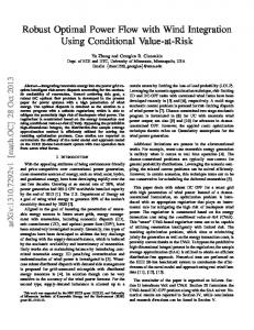
Case 1: minimum generation cost without using into account the emission level as the objective function (α=1). Case 2: equal influence of generation cost and pollution control in the objective function (α=0.5). Case 3: a total minimum emission is taken as the objective of main concern (α=0). The active powers of the 6 generators as shown in this table are all in their allowable limits. We can observe that the total cost of generation and pollution control is the highest at the minimum emission level (α=0) with the lowest real power loss (3.8144 MW). As seen by the optimal results shown in the table 3, there is a trade-off between the fuel cost minimum and emission level minimum. The difference in generation cost between these two cases (802.3646$/hr compared to 935.1502$/hr), in real power loss (9.5156MW compared to 3.8144MW) and in emission level (0.3672Ton/hr compared to 0.2176on/hr) clearly shows this trade-off. To decrease the generation cost, one has to sacrifice some of environmental constraint. The minimum total cost is at α =0.5 of the order of 969.2101$/h. The results including the voltage magnitude and the angles of three values of α shown in (Figure.3), (Figure.4) respectively. We can observe that the voltage magnitudes and the angles are between their minimum and the maximum values.
In this paper we represent two studies as follow:
1.1
TABLE III Results of minimal cost. Variables α=1 α=0.5 176.732 130.148 Pg1 48.847 57.186 Pg2 21.494 25.687 Pg5 21.688 35.000 Pg8 12.153 22.515 Pg11 12.000 19.503 Pg13 802.364 820.256 Production cost ($/hr) Emission (ton/h)
0.367
0.270
Total cost ($/h) Ploss
1004.566 9.515
969.210 6.641
α=0 68.262 71.083 50.000 35.000 30.000 32.868 935.150 0.217 1054.973 3.814
The results including the generation cost, the emission level, total cost and power losses are shown in Table III. This table gives the optimum generations for minimum total cost in three cases:
alpha=1 alpha=0.5 alpha=0
1.08 the voltage magnitude (p.u)
Case A: In this part the vector of control variables is the generated active power (5.1) x P ,P ,P ,P ,P ,P
1.06
1.04
1.02
1
0.98 0
5
10
15 buses
20
Fig.3 The voltage magnitude(p.u).
25
30
0
alpha=1 alpha=0.5 alpha=0
the voltage angle (°)
-2 -4 -6 -8
Case B: In this part the vector of control variables include the generated active power and magnitude voltage.
-10 -12
x
-14 0
5
10
15 Buses
20
25
,P
,V ,V ,V ,V ,V ,V
(5.2)
The comparisons of the results obtained by the proposed approach (FA) the case A and this case for different values of α are reported in the Table V.
Comparison with GA and PSO method
TABLE V Comparison between case B and case A case for three values of α.
The comparisons of the results obtained by the proposed approach (FA) with those found by the genetic algorithm GA [15] and particle swarm optimization [5] are reported in the Table IV. This table gives the optimum generations for minimum total cost in three cases: minimum generation cost without using into account the emission level as the objective function (α =1), an equal influence of generation cost and pollution control in this function and at last a total minimum emission is taken as the objective of main concern (α =0). TABLE IV Comparison between FA, GA and PSO.
α=1
P ,P ,P ,P ,P
30
Fig.4 The voltage angle (°).
•
The comparisons of the results between FA, GA and PSO show that the firefly algorithm gives acceptable solution .In the three cases (α =[1, 0.5, 0]), the FA gives very near results of fuel cost (802.364$/hr , 820.256 $/hr & 935.150 $/hr) compared with the results obtained with GA method (802.230$/hr , 825.003$/hr & 949.002$/hr) and in the emission level also .
Production cost ($/hr)
Emission (ton/h)
Total cost ($/h)
Ploss
FA
802.364
0.367
1004.566
9.515
GA
802.230
0.366
1003.9227
9.506
PSO
802.164
0.378
1010,4
9.728
FA
820.256
0.270
969.210
6.641
GA
825.003
0.266
968.196
6.718
PSO
820.166
0.271
969.51
6.725
FA
935.150
0.217
1054.973
3.814
GA
949.002
0.205
1061.916
3.810
PSO
935.27
0.217
1055.1
3.891
α=0.5
α=1
α=0.5
α=0
Variables
Case B
Case A
Case B
Case A
Case B
Case A
Pg1
176.775
176.732
129.952
130.148
67.888
68.262
Pg2
48.853
48.847
57.168
57.186
70.836
71.083
Pg5
21.401
21.494
25.516
25.687
50.000
50.000
Pg8
21.473
21.688
35.000
35.000
35.000
35.000
Pg11
11.978
12.153
22.408
22.515
30.000
30.000
Pg13
12.000
12.000
19.425
19.503
32.784
32.868
Production cost ($/hr)
800.783
802.364
818.14
820.25
932.777
935.150
Emission (ton/h)
0.3675
0.367
0.270
0.270
0.217
0.217
Total cost ($/h)
1003.15
1004.566
966.984
969.21
1052.27
1054.973
Ploss
9.082
9.515
6.072
6.641
3.109
3.814
α=0
The results show that, the proposed approach FA including the generated active power and magnitude voltage as variables
is lesser than proposed method FA with only the generated active power. In actual IEEE 30 bus system, the case A loss is (9.515MW, 6.641MW and 3.814MW). But, the loss in the case B is reduced to (9.082MW, 6.072 MW and 3.109 MW) for the three values of α. Also, the fuel cost and the emission is reduced as compared with case A. VI.
CONCLUSION
In this paper, a new swarm based Firefly Algorithm has been presented to solve the optimal power flow problem with emission controlled. The effectiveness of FA was demonstrated and tested with a test network of IEEE 30 bus. The results show that the FA is able to minimize the total cost along with minimization of loss in the system .A comparison with the genetic algorithm GA and particle swarm optimization PSO also has been conducted to see the performance of FA where it gives acceptable solution and he is as good as GA and PSO in solving the optimal power flow. REFERENCE [1] Hongye Wang, Carlos E. Murillo-Sanchez, Ray D. Zimmerman and Robert J. Thomas, "On Computational Issues of Market-Based Optimal Power Flow", IEEE Transactions on Power Systems, Vol. 22, No. 3, pp: 1185-1193, Aug 2007. [2] H. Talaq, Ferial and M. E. ElHawary, A summary of environmental economic dispatch algorithms, IEEE Transactions on power system, vol. 9 (3), pp 1508-1516, 1994. [3] Ruey-Hsun Liang, Sheng-Ren Tsai, Yie-Tone Chen, Wan-Tsun Tseng, Optimal power flow by a fuzzy based hybrid particle swarm optimization approach, Electric Power Systems Research, Vol.81 (2011), pp. 1466–1474 [4] X.-S. Yang, "Firefly algorithms for multimodal optimization," Stochastic Algorithms: Foundation and Applications SAGA 2009, vol. 5792, pp. 169178, 2009 [5] L. Slimani and T. Bouktir, Optimal Power Flow with Emission Controlled using Artificial Bee Colony Algorithm, 12th International conference on Sciences and Techniques of Automatic control & computer engineering, 2011, Sousse, Tunisia [6] A. J. Wood and B.F. Wollenberg. Power Generation, Operation and Control, 2nd Edition, John Wiley, 1996. [7] Glenn W. Stagg, Ahmed H. El Abiad. Computer methods in power systems analysis, McGraw-Hill, 1981. [8] L. Slimani and T. Bouktir, Economic Power Dispatch of Power System with Pollution Control using Multiobjective Ant Colony Optimization, International Journal of Computational Intelligence Research., ISSN 09731873 Vol.3, No.2, 2007, pp. 145-153. [9] B. Mahdad, T. Bouktir and K. Srairi, OPF with Environmental Constraints with Multi Shunt Dynamic Controllers using Decomposed Parallel GA: Application to the Algerian Network, Journal of Electrical Engineering & Technology, Vol. 4, No.1, 2009, pp.55-65. [10] T. Bouktir and M. Belkacemi. “Object-Oriented Optimal Power Flow”, Electric Power Components and Systems, Vol. 31 (6), 2003, pp. 525-534. [11] S. Lukasik and S. Zak, “Firefly algorithm for con-tinuous constrained optimization tasks,” in Proceedings of the International Conference on
Computer and Computational Intelligence (ICCCI ’09), N. T. Nguyen, R. Kowalczyk, and S.-M. Chen, Eds., vol. 5796 of LNAI, pp. 97–106, Springer, Wroclaw, Poland, October 2009. [12]_ X. S. Yang, “Firefly algorithm, Levy flights and global optimization,” in Research and Development in Intelligent Systems XXVI, pp. 209–218, Springer, London, UK, 2010. [13] X. S. Yang, “Firefly algorithm, stochastic test functions and design optimisation,” International Journal of Bio-Inspired Computation, vol. 2, no. 2, pp. 78–84, 2010. [14] T. Bouktir, Rafik Labdani and Linda Slimani, Economic Power Dispatch of Power System with Pollution Control using Multiobjective Particle Swarm Optimization, Journal of Pure & Applied Sciences, Vol.4, No. 2, 2007, pp. 57-77 [15] T. Bouktir, L. Slimani, M. Belkacemi, "A Genetic Algorithm for Solving the Optimal Power Flow Problem", Leonardo Journal of Sciences, Vol.4, 2004, pp. 44-58