nical Journal, 64(7):1659â1685, September 1985. [18] Stuart Campbell, Mohan Kumar, and Stephan. Olariu. The hierarchical cliques interconnection network.
Optimal Routing in Binomial Graph Networks Thara Angskun 1 , George Bosilca 1 , Brad Vander Zanden 1 , and Jack Dongarra 2 1
2
Department of Computer Science, The University of Tennessee, Knoxville University of Tennessee, Oak Ridge National Laboratory and University of Manchester {angskun, bosilca, bvz, dongarra}@cs.utk.edu
Abstract A circulant graph with n nodes and jumps j1 , j2 , ..., jm is a graph in which each node i, 0 ≤ i ≤ n − 1, is adjacent to all the vertices i ± jk mod n, where 1 ≤ k ≤ m. A binomial graph network (BMG) is a circulant graph where jk is the power of 2 that is less than or equal to n. This paper presents an optimal (shortest path) two-terminal routing algorithm for BMG networks. This algorithm uses only the destination address to determine the next hop in order to stay on the shortest path. Unlike the original algorithms, it does not require extra space for routing tables or additional information in the packet. The experimental results show that the new optimal algorithm is significantly faster than the original optimal algorithm.
1
Introduction
Recently, several high performance computing platforms have been installed with more than 10,000 CPUs, such as Blue-Gene/L at LLNL, BGW at IBM and Columbia at NASA [1]. However, as the number of components increases, so does the probability of failure. To satisfy the requirements of such a dynamic environment (where the available number of resources is fluctuating), a scalable and fault-tolerant communication framework is needed. The communication framework is important for both runtime environments of MPI libraries and the MPI libraries themselves. In general, the communication framework is based on a logical network topology. There are several existing logical network topologies that can be used in high performance computing (HPC). The fully connected topology is good in terms of fault-tolerance, but it is not scalable because of its high degree. The bidirectional ring topology is more scalable, but it is not fault-tolerant. Hypercube [2] and its variants [3–10], FPCN [11], de Bruijn [12] and its variants [13, 14], Kautz [15] and ShuffleNet [16] have a number of node restrictions. They are either not
scalable or not fault-tolerant. The Manhattan Street Network (2D Torus) [17] is more flexible (no restriction in numbers of node) than Hypercube-like topologies. However, it has a much higher average hopdistance. Variants of k -ary tree, such as Hierarchical Clique (HiC) [18] and k -ary sibling tree (Hypertree [19]) used in SFTP [20, 21], are scalable and faulttolerant. They are good for both unicast and broadcast messages. However, all nodes in their topologies are not equal (the resulting graph is not regular). Topologies, used in structured peer-to-peer networking based on distributed hash tables such as CAN [22], Chord [23], SkipNet [24], Kademlia [25], Viceroy [26], Pastry [27] and Tapestry [28], are also scalable and fault-tolerant. They were designed for resource discovery in highly dynamic environments. Hence they may not be efficiently used in HPC, owing to the overhead for managing highly dynamic applications. Binomial graph (BMG) [29] provides desirable topological properties in terms of both scalability and faulttolerance for high performance computing such as reasonable degree, regular graph (every node has the same degree), low diameter, symmetric graph (in the sense that an average inter-nodal distance is the same from any source node) and low cost factor. It also has low message traffic density, optimal connectivity, low faultdiameter, is strongly resilient and has good optimal probability in failure cases. BMG is an undirected graph G:=(V,E ) where V is a set of nodes (vertices); |V | = n; and E is a set of links (edges). Each node i, where i ∈V and i =0,1,...,n-1, has links to a set of nodes U, where U ={i ±1,i ±2,...,±2k |2k ≤ n} in circular space, i.e., node i has links to a set of clockwise (CW) nodes {(i +1) mod n, (i +2) mod n,..., (i +2k ) mod n | 2k ≤ n} and a set of counterclockwise (CCW) nodes {(n+i 1) mod n, (n+i -2) mod n,..., (n+i -2k ) mod n | 2k ≤ n}. The structure of BMG can also be classified in the Circulant graph family1 . A Circulant graph with n nodes and jumps j1 , j2 , ..., jm , where m ∈ N, is a graph 1 The family of Circulant graphs includes fully connected, ring, Recursive Circulants [30] and Midimew [31].
11
11
10
0
9
1
8
9
2
7
3
6
0
10
1
8
2
7
4
3
6
5
4 5
(a)
(b)
32
32 Torus HiC CST Hypercube Chord BMG
Torus HiC CST Hypercube Chord BMG
16 Diameter (Hops)
16 Average Distance (Hops)
in which each node i, 0 ≤ i ≤ n − 1, is adjacent to all the vertices i ± jk mod n, where 1 ≤ k ≤ m. BMG is a Circulant graph where jk is the power of 2 that is less than or equal to n. For a BMG of size n (having n nodes), each node has a degree δ (number of neighbors) as shown in Equation (1). (2 × dlog2 ne) − 1 For n = 2k , where k ∈ N (2 × dlog2 ne) − 2 For n = 2k + 2j , δ= where k, j ∈ N ∧ k 6= j 2 × dlog2 ne Otherwise (1) Figure 1(a) illustrates an example of a 12-node binomial graph, where the thin lines represent all the connections in the network. The other way to look at the binomial graph is that it is a topology, which is constructed from merging all necessary links being able to create binomial trees from each node in the graph. Figure 1(b) shows an example of a binomial tree where node 0 is the root node. The arrows point in the direction of the leaf nodes. Obviously, BMG is able to deliver broadcast messages optimally from any node within dlog2 (n)e steps because of its capability to create the binomial tree out of each node.
8
4
8
4
2
2
1
1 16
32
64
128
256
512
16
1024
32
64
128
256
512
1024
Number of Nodes
Number of Nodes
(a)
(b)
Figure 2. Distance Comparison. (a) Average ¯ (b) Diameter (D). distance (d).
This paper introduces an optimal (shortest path) two-terminal routing algorithm for BMG networks. This algorithm uses only the destination address to determine the next hop in order to stay on the shortest path. Unlike the original algorithm, it does not require extra space for routing tables or additional information in the packet. In fact, the shortest-path problem for Circulant graphs of arbitrary degree is NP-hard [32]. There are several optimal algorithms for specific types of Circulant networks such as 2-Circulant [33, 34] and Recursive Circulant Networks [35]. However, these algorithms can not be directly applied with the BMG, due to their restriction with constant degree. Actually, BMG and the undirected Chord [36] are exactly the same topology when the number of nodes is a power of two2 . Hence, the optimal routing in the undirected Chord [36] may also be used in BMG. Figure 3(a) il¯ overhead (in percent) lustrates an average distance (d) of an undirected chord routing algorithm. The percent d¯ −d¯Optimal overhead was calculated from Chord × 100. d¯ Optimal
Figure 1. Binomial graph structure. (a) 12node BMG. (b) Binomial tree from node 0.
d¯ =
Pn−1 Pn−1 x=0
y=0 d(x, y)
n × (n − 1)
, where x 6= y
(2)
The average distance and diameter of BMG, along with related network topologies, are shown in Figure 2(a) and Figure 2(b), respectively. The results indicate that BMG has the lowest average distance (≈ log23(n) ) and diameter (O(d dlog22(n)e e)) among them.
Histogram 100% 25
50% Diameter Overhead (Hops)
%Average-Distance Overhead
The distance d (x,y) between node x and node y in a graph is defined as the length of the shortest path from x to y in the graph. The diameter D of a graph is given by max(d (x,y)) over all possible pairs (x,y) of nodes in the graph. The diameter D is the longest of the shortest paths between any two nodes in the graph. The average distance d¯ of a graph is given by Equation (2).
30
20 15 10 5
2
0% 0
1
2
1
0
0
16
32
64
128 256 512 Number of Nodes
(a)
1024 2048 4096
16
32
64
128
256
512
1024 2048 4096
Number of Nodes
(b)
Figure 3. Performance of undirected chord routing algorithm on BMG topology. (a) d¯ overhead (%). (b) D overhead (hops). This figure indicates that an undirected chord rout2 if
the number of nodes in the undirected Chord is not power of two, it will create roughly the same small groups of nodes such that the number of groups is a power of two and will use their routing algorithm [36] between those groups.
ing algorithm is not optimal for BMG unless the number of nodes is a power of 2 or middle points between the power of 2 (e.g., 24, 48, 96, ...). Figure 3(b) illustrates diameter (D) overhead in the number of hops (i.e., DChord − DOptimal ). The structure of this paper is as follows. Section 2 describes the original routing algorithm. The new optimal routing algorithms are discussed in section 3. Section 4 presents the experimental evaluations, followed by conclusions and future work in section 5.
2
Original routing algorithms
This section presents three original two-terminal routing algorithms [29]. One optimal routing algorithm is based on breadth-first search, and the two suboptimal routing algorithms are called basic and variant. Each node in the graph may run the same routing algorithm because all nodes in BMG are equal (both regular and symmetric).
2.1 Breadth-First Search Optimal Algorithm The optimal routing algorithm can use a breadthfirst search technique with a modified graph coloring algorithm. Although this algorithm gives the optimal result, the complexity of the algorithm is O(δ D ). Instead of recomputing the next hop in every message transmission, the breadth-first search technique can use a routing table to keep the result of the next hop sorted by the shortest path from the node itself to all other nodes in BMG. However, the routing table requires an extra space of O(n2 ).
2.2 Basic Sub-Optimal Algorithm A basic algorithm to estimate the shortest path between nodes is to use a rule-based method that sends the unicast messages to a neighbor that has the closest ID to the destination ID as shown in Algorithm 2. The complexity of the basic unicast routing algorithm is O(δ). The experimental results indicate that the basic is a sub-optimal algorithm (i.e., average distance overhead 6= 0) as shown in Figure 4.
Algorithm 1 Finding an Optimal Route with Breadth-First Search Require: 1 ≤ myID ≤ n ∧ 1 ≤ destID ≤ n, n ∈ N 1: for i = 0 to n do 2: State[i] ⇐ INIT 3: end for 4: State[myID] ⇐ START 5: enQueue(myID) 6: while Queue is not empty do 7: nodeID ⇐ deQueue() 8: if nodeID = destID then 9: break 10: end if 11: Get neighborID of the nodeID 12: for i = 0 to (N umbersof neighbor) − 1 do 13: if State[nodeID] = INIT then 14: State[neighborID[i]] ⇐ START 15: Parent[neighborID[i]] ⇐ nodeID 16: enQueue(neighborID[i]) 17: end if 18: end for 19: State[nodeID] ⇐ DONE 20: end while 21: nodeID ⇐ destID 22: while Parent[nodeID] 6= myID do 23: nodeID ⇐ Parent[nodeID] 24: end while 25: Return nodeID Algorithm 2 Find neighborID which has the estimated shortest distance to destID Require: 1 ≤ myID ≤ n ∧ 1 ≤ destID ≤ n, n ∈ N 1: Min ⇐ ∞ 2: Get neighborID of myID 3: for i = 0 to (N umbersof neighbor) − 1 do 4: Distance ⇐ |destID − neighborID[i]| 5: if Distance < Min then 6: Min ⇐ Distance 7: nextHopID=neighborID[i] 8: end if 9: end for 10: Return nextHopID 12
Basic Variant
Histogram
Basic Variant
100%
10
Diameter Overhead (Hops)
This algorithm is the variant of the basic algorithm that allows messages to go forward to a neighbor of which ID is not the closest ID to the destination ID if the destination is directly connected to the neighbor. The complexity of the variant unicast routing algorithm is O(δ 2 ). Figure 4(a) and Figure 4(b) present the overhead of both sub-optimal algorithms. They depict that the variant algorithm is marginally better than the basic algorithm in terms of d¯ and D.
%Average-Distance Overhead
50%
2.3 Variant Sub-Optimal Algorithm
8 6 4 2
2
0% 0
1
2
1
0
0 16
32
64
128 256 512 Number of Nodes
(a)
1024 2048 4096
16
32
64
128
256
512
1024 2048 4096
Number of Nodes
(b)
Figure 4. Sub-optimal routing performance. (a) d¯ overhead (%). (b) D overhead (hops).
3
New routing algorithms 1 2
In order to always stay on the shortest path from a source to a destination, messages must be delivered through a neighbor that has the estimated shortest hop to the destination unlike the original basic sub-optimal algorithm that estimates the shortest distance between neighbors and destination (i.e., a greedy algorithm). The key to success of this algorithm is how well we can estimate the number of hops that is used for sending messages between two nodes. Several methods to calculate the number of hops between two nodes have been explored as follows.
3 4 5 6 7 8 9 10 11 12 13
3.1 Bit Counting method
i n t l o ok u p 8 ( unsigned { return LTB8 [ n LTB8 [ ( n>>8) LTB8 [ ( n>>16) LTB8 [ ( n>>24) }
int n) & & & &
0 xffu 0 xffu 0 xffu 0 xffu
] ] ] ]
+ + + ;
Figure 5. 8-Bit Lookup Table for 32-bit Architecture
than the parallel counting techniques, however they require extra memory to store the table. Figure 6(a) and Figure 6(b) present the d¯ and D overhead of the bit counting method. They emphasize that the bit counting method is sub-optimal. 40
5 Histogram 50% Diameter Overhead (Hops)
35 %Average-Distance Overhead
The bit counting method represents the distance between a source and a destination in a binary format. The bit-1 represents the number of hops that messages can travel, e.g., if a distance between a source and a destination (|destID −srcID) is 9 (binary is 1001), a message is forwarded to nodes with distance 8 (1000) and 1 (0001). Hence the message can be delivered within two hops. From the above example, it does not matter which of the distances is selected as the first hop. Thus, load balancing of both links and neighbors can be implemented by a node if the next neighbor is randomly selected from all those candidates. Quality of service (QOS) can also be implemented by a node simply by selecting the next hop based on the priority of its candidate neighbors. The bit counting method can be used to estimate the number of hops by counting the number of bit-1 of distance between the source and the destination in both clockwise and counter-clockwise directions. The estimated number of hops is the minimum number of bit of both directions. The complexity of this algorithm is O(1). In practice there are several fast bit counting algorithms (O(1)). They can be divided into two classes. The principal idea of the first class is to count the number of bits in parallel fashion. These algorithms re-arrange an original binary number into several small groups of bits, then count the number of bits in each group simultaneously and finally sum the results. An example of an algorithm in this class is the MIT HAKMEM item 169 [37]. The second class is based on a lookup table of pre-computed bit counting. Figure 5 illustrates an example of the 8-bit lookup table. The LTB8 holds the number of bit-1 of every value (0-255) for an 8-bit number. Counting the bit of a 32-bit integer can be performed by masking out four sets of eight bits in the given integer and indexing them into the LTB8 array. Then, the final result is the sum of results of every set of eight bits. Methods based on the lookup table also have complexity O(1). They might be faster
s t a t i c i n t LTB8 [ 2 5 6 ] = { 0 ,1 ,1 ,2 ,1 ,2 ,2 ,3 ,... ... ,5 ,6 ,6 ,7 ,6 ,7 ,7 ,8 };
30 25 20 15 10
25%
4
0% 0 1 2 3 4 5 3
2
1
5 0
0 16
32
64
128 256 512 1024 2048 4096 Number of Nodes
(a)
16
32
64
128 256 512 1024 2048 4096 Number of Nodes
(b)
Figure 6. Performance of the bit counting method. (a) d¯ overhead (%). (b) D overhead (hops). The average and maximum values of the overhead of d¯ and D for the bit counting method in a configuration between 16 and 4096 nodes compared with the original algorithms, basic and variant sub-optimal are shown in Table 1 and Table 2. Estimating the number of hops by a simple bit counting method does not seem to be a good idea. However, it is worth mentioning in this section, since it will be used in the subsequent section.
3.2 Consecutive Bit Elimination Method Estimating the number of hops using the bit counting method might be too pessimistic, e.g., if a distance between a neighbor and a destination (|destID − neighborID|) is 7 (binary is 0111), the bit counting method will estimate the number of hops is 3, jumping
Table 1. d¯ Overhead comparison Values (%) Algorithms Average Maximum Basic 5.555140 11.3849 Variant 4.692380 10.5893 Bit Counting 25.1307 36.2324 Con. Bit Elimination 1.28199 4.43152
The complexity of this algorithm is O(log2 (n)). An implementation of this algorithm can be done by simply scanning and transforming a given log2 (n) bit distance from right to left using a state diagram as shown in Figure 7, where di is an original distance and qi is a distance in the opposite direction. The label on each transition between states is written in the form of input/output (i.e., Mealy machine). di = 0 / qi = 0
di = 0 / qi = 0
Table 2. D Overhead comparison Values (Hops) Algorithms Average Maximum Basic 0.454055 2 Variant 0.449155 2 Bit Counting 2.23254 5 Con. Bit Elimination 0.351139 2
di = 1 / qi = 0 OFF
FIRST_ONE
di = 0
di = 0
DONE
di = 0
di = 0 / di = 1 qi = 0
di = 1 / qi = 0, qi-1 = 1 di = 0, di-1 = 0
CLUSTER
di = 1 / di = 0
to nodes with distance 4 (0100), 2 (0010) and 1 (0001), respectively. However, by using the counter-clockwise links we can use only 2 hops by jumping to distance 8 (1000) on one direction and 1 (0001) on the other direction (7 = 8-1). Hence we may estimate more precisely the number of hops between two nodes by eliminating the sets of consecutive bits before counting the number of bits in both directions. Consecutive bits elimination can be performed by adding the value of the least significant consecutive bit to the distance between source and destination in both clockwise (CW) and counterclockwise (CCW) directions. This procedure is repeatedly performed until there is no consecutive bit left or the result after adding the values is more than jm , where jm is a maximum power of 2 that is less than or equal to n. For example, a distance in clockwise direction is 110 (the binary is 1101110), i.e. CW = 110 and CCW = 0. Consider the distance binary 1101110, the first group of consecutive bits from the right is 1110; therefore, the least significant, consecutive bit is 2 (binary is 10). The first step is performed by adding 2 (10) to both CW and CCW directions. Hence, the distance 110 can be routed by jumping with distance 112 (binary is 1110000) in CW and 2 (binary is 10) in CCW. Notice that the binary of 112 (1110000) still has a consecutive bit, thus the next value to add in both directions is 16 (binary is 10000). After adding 16, distance 110 can be jumped with distance 128 (binary is 10000000) in CW and 18 (binary is 10010) in CCW. In conclusion, the routing for a distance of 110 in the clockwise direction can be performed within three hops, i.e., one jump in a clockwise direction with the distance 128 and two jumps in a counter-clockwise direction with the distance 2 respectively 16. Again, it does not matter the order in which these jumps are undertaken. Thus, the load balancing and quality of service can be implemented as mentioned in section 3.1.
Figure 7. A state diagram to perform bit transformation Unfortunately, eliminating consecutive bits is difficult to do in constant time using parallel bit transformation because of the dependency between bits. However, this method can be improved by scanning only part of the entire log2 (n) bits as shown in Figure 8. 1 2 3 4 5 6 7 8 9 10 11 12 13
static i n l i n e int check 11 ( int d) { int p r e v l s f , l s f ; p r e v l s f =−1; while ( d ) { l s f = ( d & −d ) ; i f ( ( p r e v l s f