Optimal Server Resource Allocation Using an Open ... - CiteSeerX

Optimal Server Resource Allocation Using an Open Queueing Network Model of Response Time Alex Zhang, Pano Santos, Dirk Beyer, Hsiu-Khuern Tang Intelligent Enterprise Techno logy Laboratory HP Laboratories Palo Alto HPL-2002-301 October 21st , 2002* service level agreement, web performance tuning, software performance modeling, response time, queueing, optimization

We present a nonlinear integer optimization model for determining the number of machines at each tier in a multi-tier server network. We utilize a result from an open queueing network model on the average response time; the optimization model is to minimize a weighted sum of total machines while satisfying the average response time constraint (or a service level expression that is convertible to the average response time). We then discuss the solution to this optimization model and present an algorithm that utilizes a bounding procedure.

* Internal Accession Date Only  Copyright Hewlett-Packard Company 2002

Approved for External Publication

1 Introduction This report examines the issue of dynamically provisioning computing resources, in the form of server machines, to meet a prescribed service level on average response time. This issue frequently arises in ASPs (Application Service Providers) and in web-service operations (e-commerce sites, for example). The web-service system that we consider has a tiered structure. Typically three tiers are con gured: web servers, application servers, and database servers. Within each tier, multiple machines can be provisioned to share the incoming workload which consists of a series of dierent types of web requests. The response time is de ned in this report to be the time taken for a web request to go through the three-tiered system (i.e. \server-side response time"). Our question is to allocate an adequate number of machines to each tier in order to meet certain service level requirement. Applications that allow dierent number of machines at each tier are called horizontally scalable. We deal with such a horizontally scalable system where service level requirement is expressed in average response time of the system. Since the system response time is the sum of response times at each of the three tiers, the service level requirement can be met by dierent con gurations in the number of machines at each tier. For example, the con guration of 3 web servers, 2 application servers, and 1 database server may achieve the same average response time as the con guration of 1 web server, 3 application servers, and 1 database server. The question, then, is to nd a minimum number of machines in total to meet a prescribed service level requirement. Realizing that machines at dierent tiers might be dierent and incur dierent costs, the more general optimization problem is to minimize the total weighted sum of the machines, with the weights re ecting the \costs" of some kind (such as operating costs) of machines at dierent tiers. This problem is a sub-problem in a more general problem of web transaction analysis and optimization (TAO) discussed in HPL Technical Report HPL-2002-45 (Garg et al 2002). We refer to this report for a more detailed discussion of the system and modeling eorts. Appleby et al (2001) describe various aspects of IBM's Oceano project which is centered on service level management and which includes many issues that the TAO project also sets out to solve. Menasce and Almeida (1998) present general issues in capacity planning issues for web performance. In another HPL technical report HPL-2002-64, Santos, Zhu and Crowder (2002) address the issue of allocating resources (machines) in a tree-like topology of a data center, 2

considering performance constraints such as link bandwidth and switch capacity while minimizing communication delay between the assigned servers. They propose a mathematical optimization model with binary variables for optimally con guring the topology. This report diers from Santos et al (2002) in that we consider only the average response time performance measure. Our topology is a tiered structure. The use of the queueing model in expressing the average response time leads to a general non-linear integer problem, but with only a few general integer variables. These simpli cations allow us to characterize the solution of the problem and devise an algorithm to nd the solution eciently. We point out that the solution of the problem is relevant to the dynamic resource allocation at a Utility Data Center (UDC). The dynamic resource allocation at a UDC requires the integration of demand and capacity planning. This concept is known as Capacity on Demand. Capacity on Demand consists of optimizing the assignment of buers (or shared) resources to satisfy the requirements of multiple applications. A UDC enables multiple applications to be hosted on a collection of shared resources, where the resources assigned to the applications may be increased when workload increases and reduced when workload reduces. This dynamic resource allocation allows exible service level agreements (SLAs) in an environment where peak workload is much greater than the normal steady state. A key problem with Capacity on Demand is that the user needs are translated into a logical con guration, and physical resources are then assigned to the logical con guration to satisfy the resource requirements of the application. The problem addressed in this paper is precisely to determine the optimal resource requirements of an application under a workload in such a way that application SLAs are satis ed. This report is organized as follows. We will next describe the queueing model which gives the expected (average) response time as a function of demand and the amount of resources allocated. In Section 3, we will then formulate the resource allocation problem as a mathematical program consisting of a linear objective function and a nonlinear constraint, with general integer decision variables. Sections 4 and 5 examine the twotier problem and the general n-stage problem, and give the main mathematical results on feasibility conditions, bounds, and relaxed problem solutions. Section 6 presents our main algorithmic results on solving the practical integer optimization problems. In Section 7, we show that our optimization model is applicable to any service level metric that can be translated into the average response time.

3

2 A Queueing Model of Response Time In HPL-2002-45, we have modeled the 3-tiered web system as an open queueing network, with a single type of critical resource (such as CPU). Related work addressing systems performance predictions on queueing time is the layered model by Rolia and Sevcik (1995), and Shiekh et al (1997). Here we present a simple (non-iterative) model for queueing time. Its simplicity is a computational advantage when used as input in an optimization routine which needs to determine the optimal resource allocation frequently and quickly. In our simple model, each machine is modeled as a processor sharing queue. Assuming that all machines at the same tier are identical, and that the workload balancing and scheduling is such that the workload is shared equally among the machines at the same tier, this queueing model gives the average response time of the 3-tier system as follows: E [S ] E [S ] E [S ] E [R] = + + (1) 1 ;  E [S ]=N 1 ;  E [S ]=N 1 ;  E [S ]=N where E [S ], E [S ], and E [S ] are the expected processing times (or service demands) of a request on the critical resource (such as CPU) at web, application and database tiers, respectively;  ,  , and  are the arrival rates to the three tiers (e.g.  is the total arrival rate to all the web servers in the web tier); and N , N and N are the number of servers in each of the three tiers, respectively. The only inputs to the average response time model are the arrival rates (or throughput) ( ,  ,  ), the number of servers at each tier (N , N , N ), and the average service times (E [S ], E [S ], E [S ]). The average service times (service demands) can be computed from the measured utilization rates of the critical resource (CPU), through the following relationship: E [S ] = U =( =N ); where U < 1 is the measured per-machine average utilization rate; ( =N ) is the permachine average throughput rate. We have tested the accuracy of the average response time formula (1) using measured response time data recorded from a test bed (the \PetStore" e-tailing web site, see Garg et al 2002) consisting of 1 web server, 2 application servers, and 1 database server. The data log also includes CPU utilization percentages for all machines in 5-minute intervals. Under various workload scenarios (dierent levels of request intensity and dierent mix percentages of request types), the queueing formula (1) was found to be from 4% to 27% of the actual average response time. 1

1

1

1

2

1

2

1

2

3

2

2

3

2

2

3

1

3

1

1

2

3

3

1

1

3

2

2

3

3

3

1

1

1

1

1

1

4

1

3 Resource Allocation with the Average Response Time Measure Our model of resource optimization would then be to minimize a total weighted \cost" (represented by machine replacement cost or operating cost) of the system, subject to the constraint that the average system response time to be less than or equal to a certain level (T , such as 1 second). That is: min

N1 ;N2 ;N3

s.t.

h1 N1 + h2 N2 + h3 N3

(2)

E [S1 ] E [S2 ] E [S3 ] + + 1 ; 1E [S1]=N1 1 ; 2E [S2 ]=N2 1 ; 3E [S3 ]=N3 N1 ; N2 ; N3 positive integers; E [R] =

 T ; (3)

where weights h , h , and h (all assumed to be strictly positive) are to re ect the dierence in the costs of the dierent servers; for example, if a database server machine is twice as expensive as a web server machine, then h = 2
h . As we mentioned earlier, if costs are dicult to ascertain, a convenient simpli cation would be to minimize the total number of machines (N + N + N ); i.e. to set h = h = h = 1. When N increases, the values of  and E [S ] remain the same, as  is the aggregate arrival rate to the web tier. Hence, parameters  ;  ;  and E [S ]; E [S ]; E [S ] are true input parameters in the optimization model. Finally, although we have given the explicit formulation for the 3-tiered system, we could easily generalize the formulation to any n-stage system (each tier is a stage). However, we will begin our discussion about the solution of the optimization model with the two-stage model. 1

2

3

3

1

1

2

3

1

1

1

2

3

1

1

1

2

3

1

2

3

4 The Two-Stage System If the number of servers at a particular tier is xed (say there can be only one database server), the optimization problem is simpli ed. The 2-stage problem provides a case for mathematical examination. Consider the 2-stage version of this problem: min

N1 ;N2

s.t.

h1 N1 + h2 N2 s1 s2 + 1 ; u1=N1 1 ; u2=N2

5

(4)

 T;

(5)

N1 ; N2 positive integers:

where s  E [S ] and u   E [S ] are input parameters. Here u can be interpreted as an expression of workload; for example, u = 1:5 signi es that the aggregate workload on web server tier is equivalent to 1.5 web server machines working full time (at 100% utilization). Clearly, we can also replace the non-negativity constraints N ; N positive integers by a tighter N  max(u ; 1) and N  max(u ; 1). The basic tradeo expressed through the above optimization problem is that of balancing fewer expensive machines with a resulting longer response time against more numerous cheaper machines with a resulting shorter response time. We rst look at the feasibility of this simple optimization problem. Proposition 1. The 2-stage problem is feasible if and only if s + s < T . Proof. Say s + s < T . Then let N ! 1 and N ! 1, we have s s + 1 ; u =N 1 ; u =N ! s + s < T: i

i

i

i

i

i

1

1

1

1

2

2

1

1

2

1

2

2

1

2

1

2

1

2

1

2

2

Hence the constraint can be satis ed by large N and N ; the problem is feasible. Now assume that the problem is feasible. Then there exist positive integers N and N such that s s +  T: 1 ; u =N 1 ; u =N Hence, s s +  T: s +s < 1 ; u =N 1 ; u =N 1

2

0 1

1

2

0 1

1

1

0 2

2

2

1

2

1

0 1

2

0 2

We also nd lower bounds on the feasible N and N : Proposition 2. The feasible N and N satisfy u (T ; s ) N > ; N > u (T ; s ) : 1

1

1

k

2

2

1

2

T ; s1 ; s2

2

1

2

1

2

s1 1 ; u1=N1 < T ; s2; u (T ; s2 ) N1 > 1 : T ; s1 ; s2

6

1

T ; s1 ; s2

2

Proof. From the feasibility condition, s T + s 1 ; u =N 1 ; u =N 1

0 2

2

>

s1 +s ; 1 ; u1=N1 2

(6)

k

Similar derivation for the inequality for N . 2

Remark. Since N and N are required to be integers, we can tighten the inequality to u (T ; s ) N d e where dxe stands for the smallest integer greater than or equal to x. T ;s ;s 1

1

1

2

2

1

2

Example. Let s = 0:3, s = 0:5, u = 0:3, u = 0:4, T = 1. Notice that s + s = 0:8 < 1

2

1

2

1

2

T = 1, hence the necessary and sucient condition for feasibility of the optimization

problem is satis ed. Then

0:3(1 ; 0:5) = 0:75; N  1; 1 ; 0:3 ; 0:5 0:4(1 ; 0:3) = 1:4; N  2: N > 1 ; 0:3 ; 0:5 N1 >

1

2

2

k The bounds on N and N will facilitate the numerical search for the optimal values. In general, the numerical search will have to enumerate all integer pairs (N ; N ) satisfying Proposition 2. In section 6, we will give an iterative algorithm for tightening these bounds, which we will utilize in an algorithm for obtaining the integer optimal solution. The continuous-variable version of the optimization problem, however, has a closed form solution. Proposition 3. The continuous-variable version of the 2-stage problem has the following optimal solution: 1

2

1

2

q N1 = u1 + s1 u1 =h1 ; q N2 = u2 + s2 u2 =h2 ; c

c

where > 0 is the shadow price of the required average response time and is given by p p p = h s u + h s u : 1 1

1

2 2

T ; s1 ; s2

The objective function value is given by

p

Z = h1 u1 + h2 u2 + c

q

Proof. Consider the Lagrangian:

2

 q s1 u1 h1 + s2 u2 h2 :

! s1 s2 L(N1 ; N2 ; ) = h1 N1 + h2 N2 + + : 1 ; u1=N1 1 ; u2=N2

7

Take partial derivative w.r.t. N and set to zero we obtain: 1

@L s1 u1 = h1 ;
@N1 (N1 ; u1)2 = 0;

hence

q N1 = u1 + s1 u1 =h1 : c

Similarly we obtain N . Since N and N are continuous, the constraint c

c

2

c

1

2

s1 + s2 1 ; u1=N1 1 ; u2=N2

T

must be binding (= T ); substituting N and N into the equality and simplify algebraically we can solve for . k c

c

1

2

Remark. Proposition 1 guarantees T ; s ; s 1

N1 > u1 and N2 > u2 . c

2

> 0 if the problem is feasible. Also,

c

Example (continued). Let s = 0:3, s = 0:5, u = 0:3, u = 0:4, T = 1. Introduce 1

2

1

2

h1 = 1, h2 = 2. We solve the continuous-variable version of the 2-stage problem as

follows.

p p p = ph s u + ph s u = 1
0:3
0:3 + 2
0:5
0:4 = 4:6623; Tq; s ; s 1q; 0:3 ; 0:5 N = u + s u =h = 0:3 + 4:6623 0:3
0:3=1 = 1:6987; q q N = u + s u =h = 0:4 + 4:6623 0:5
0:4=2 = 1:8743; 1 1

1

2 2

1

c

1

c

2

Z

c

1

2

2

2

1

1

1

2

2

2

= h N + h N = 5:4473: 1

c

1

2

c

2

The integer-optimal solution (found through enumeration) is N  = N  = 2, with achieved average response time of 0.978 seconds (better than the required T = 1 second), and objective function value of 6 (worse than 5.4473 of the continuous solution). 1

2

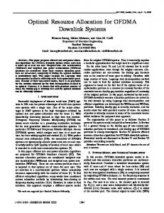
k From Proposition 3, the continuous-variable solution of the problem has some interesting properties. The shadow price ( ) of the required average response time is the increase in the objective function value (cost) per unit of decrease on the response time; for example, \ = $20/second" denotes that each second in decreased response time will cause an approximately $20 increase in the total objective function value (cost). The shadow price as an output of the mathematical optimization model may have pricing 8

gamma 80 60 40 20

1.2

1.4

1.6

1.8

2

T

Figure 1: Shadow price for the required average response time T . Parameters: s = 0:3, s = 0:5, u = 0:3, u = 0:4, h = 1, h = 2. 1

2

1

2

1

2

implications on SLAs. We notice that the shadow price is related to T by the following relationship: / 1=(T ; c) (where c  s + s ). The shadow price decreases rapidly as the allowable response time increases. On the other hand, the number of machines at each tier, as well as the objective function value (cost), is approximately inversely proportional to the required response time (N / 1=(T ; c); Z / 1=(T ; c)). Figure 1 and Figure 2 show the relationship of , N and N as a function of the required response time T . 2

1

2

c

c

i

c

c

1

2

5 The General Case: An n-Stage System All three propositions in the 2-stage system case can be generalized to n-stage systems. Here are the restatements of the old results. Proposition 1. The n-stage problem is feasible if and only if P s < T . Proposition 2. The feasible N , i = 1; 2; : : : ; n, satisfy P u (s + T ; s) N > : (7) P T; s n

i=1

i

i

n

i

j =1

i

i

j

n

j =1

j

Proposition 3. The n-stage problem has the following continuous-variable solution: N

c

i

q

= u + s u =h ; i

i

9

i

i

(8)

N1,N2 3 2.5 2 1.5 1 0.5 1.2

1.4

1.6

2

1.8

T

Figure 2: N (lower curve) and N (top curve) as a function of the required average response time T . Parameters: s = 0:3, s = 0:5, u = 0:3, u = 0:4, h = 1, h = 2. c

c

1

2

1

2

1

2

1

2

where > 0 is the shadow price of the expected response time and is given by

p = P

n

i=1

T;

The objective function value is Z = c

X n

P

i

i

i

=1 s

i

n i

p

hu + i

i=1

ph s u

(9)

:

i

Xq suh: n

i

i

(10)

i

i=1

6 The Integer Program: A Solution Algorithm We point out that the continuous-variable version of the problem is only a relaxation of the original integer problem. We emphasize that the integer optimal solutions might be far away from the continuous solutions as given by equation (8); that is, if the continuous solution is (N ; N ) = (1:44; 1:79), the integer optimal solution might be (1; 4). Rounding up each of the continuous N will clearly lead to a feasible, but not necessarily optimal, solution. Proposition 2 gives a lower bound on each N , and can be utilized as the starting values in a numerical search algorithm. The following proposition further gives a (dynamic) upper bound on the search. Proposition 4. If (N ; : : : ; N ) are integers and satisfy the expected average response time constraint, then any other integer solutions (N ; : : : ; N ), where N  N for all i 1

2

i

i

0 1

0

n

1

10

n

i

0

i

with strict inequality for at least one i, cannot be optimal. Proof. Suppose integers N  N for i = 2; : : : ; n, with N > N . Then (N ; N ; : : : ; N ) is a feasible integer solution, since the average response time E [R] is strictly decreasing in each N . However, P h N > P h N ; hence (N ; N ; : : : ; N ) cannot be optimal. 0

i

n

i=1

i

0

n

i

0 1

1

i

i=1

i

i

1

i

1

2

2

n

n

k

We further obtain bounds on the integer-optimal objective function values (costs). Proposition 5. Let Z  be the integer-optimal objective function value, and N be the continuous-variable solution as given by (8) with objective function value Z as given by (10). Then c

i

c

X n

hN i

c i

i=1

 Z  Z  Z  c

UB

X n

h dN e:

i=1

(11)

c

i

i

Proof. Since the continuous-variable model is a relaxation of the integer model, we have Z  Z . Since each dN e  N , the integer solution (dN e; dN e; : : : ; dN e) is a c

c

c

i

i

c

c

1

c

2

n

feasible solution since the response time function (the left-hand-side of the constraint) is decreasing in each N . Hence the second inequality holds. k i

For the previous numerical example introduced in previous sections, N = 1:6987, N = 1:8743, and Z = 5:4473, hence Proposition 5 yields the bounds 5:4473  Z   6 (the true Z  = 6). Figure 3 illustrates the use of Proposition 5 in bounding the integer optimal solution. To provide a heuristic solution to the integer model, we rst solve the continuous-variable problem (in closed-form), and simply round up each N if N is not an integer (i.e. to the next higher integer), we will obtain an integer feasible solution, with a guaranteed performance within Z ; Z = P h (dN e ; N ) from the true optimum. When N , i = 1; 2; : : : ; n, are relatively large (say greater than 3), the relative gap between the heuristic solution and the true integer optimal solution is quite small. c

c

1

2

c

UB

c

n

i=1

i

c

c

i

i

c

c

c

i

i

i

6.1 Improved Bounds with an Iterative Procedure Proposition 5 is useful in the search for integer optimal solution in that we know any integer optimal solution must satisfy h N +h N +


+h N  Z ; hence if N ;


; N ; have been determined, we must have N  (Z ;h N ;


;h ; N ; )=h . This narrows the search range in the n-th dimension (N ). 1

1

2

c

n

n

11

2

n

1

1

c

n

n

1

1

n

1

n

n

1

Figure 3: An illustration of the lower and upper bounds Proposition 5 also enables us to improve the bounds as given by Proposition 2. The procedure is as follows. Step 0. Step 1.

P u (s + T ; =1 s ) e: (Initial lower bounds) Following Proposition 2, set N = d T ; P s =1 (Upper bounds) For i = 1; 2; : : : ; n, obtain an upper bound on N by using the inequality N  (Z ; P 6= h N )=h  (Z ; P 6= h N )=h . Set N = b(Z ; P 6= h N )=h c. (Improved lower bounds) For i = 1; 2; : : : ; n, obtain X an improved lower s bound on N by using the inequality 1 ; u =N + 1 ; su =N  T 6= where for j 6= i, N is set to its upper bound N . Set new N = d 1 ; (us =t ) e where t  T ; P 6= 1;( j j jUB ) . (Improved bounds) If for some i, the new N is better (greater) than the old N , then replace all old bounds by the new bounds and go back to Step 1; Otherwise, stop and output the current N and N . n

i

j

j

i

n

j

j

i

i

UB

j

UB

j

i

Step 2.

i

LB

i

j

i

LB

j

j

UB

i

j

LB

j

i

j

i

i

j

i

j

i

i

j

i

j

j

i

j

UB

LB

j

i

s

i

Step 3.

i

i

j

i

i

u =N

LB

i

LB

i

LB

UB

i

i

The above algorithm uses the service level constraint (on average response time) to nd the lower bounds, and then in turn uses the optimality condition P h N  Z to n

i=1

12

i

i

UB

nd the upper bounds. The upper bounds may lead to improved lower bounds from the response time constraint; the iteration terminates when no further improvements can be made. We illustrate the above bounding algorithm using the previous numerical example (where n = 2). Recall s = 0:3, s = 0:5, u = 0:3, u = 0:4, h = 1, h = 2. 1

2

1

2

1

2

Step 0. From Proposition 2, N = 1; N = 2. Step 1. Upper bounds. N  6 ; 2N = 6 ; 2
2 = 2; hence N = 2. N  (6 ; N )=2 = (6 ; 2)=2 = 2; hence N = 2. (Since N = N = 2, we have N = 2.) Step 2. Improved lower bounds. t = T ; ; 2 2 2UB = 1 ; ; = 0:375; N = d ; 11 1 e = d ; e = d1:5e = 2 (an improvement). Further iterations do not improve the current bounds, hence the procedure terminates with N = N = N = N = 2. In this numerical example, the bounding procedure happens (by chance) to lead to the unique optimal integer solution (without applying any optimization procedure). LB

LB

1

2

LB

1

UB

2

1

LB

2

UB

1

LB

2

UB

2

2

2

s

1

1

(s

)

=t

1

LB

UB

1

(u

1

)

=N

0:5 (0:4=2)

0:3 (0:3=0:375)

u

LB

1

1

LB

1

UB

2

2

6.2 A Numerical Search Algorithm We rst give a simple algorithm for solving the integer optimization problem with n = 2 (two tiers). We then give a recursive algorithm for solving a general n-stage problem. Algorithm TwoStage(T ): Given a required average response time T , nd the optimal N and N to minimize h N + h N . 1

2

1

1

2

2

Step 0. Feasibility test: If s + s  T then the problem TwoStage(T ) is infeasible. Terminate and output \infeasible". Step 1. Bounds: Compute the continuous-variable solution from equations (8), (9) and (10). Compute the lower and upper bounds N and N for i = 1; 2; : : : ; n following the iterative bounding procedure outlined in the previous section. Set the optimal objective function value Z to in nity. Step 2. Set N to its lower bound N . Step 3. Set t = (T ; ; 11 1 ) and N = d ; 22 2 e. Step 4. Compute objective function value h N + h N . If this is lower than Z , then set Z = h N + h N and remember (N ; N ). 1

2

LB

1

2

1

s

1

u

2

u =N

1

(s

1

1

1

2

2

=t

1

)

2

2

1

13

2

LB

UB

i

i

Step 5. If N < N then increment N by one and return to Step 3; otherwise terminate and output (N ; N ). UB

1

1

1

1

2

To explain the above TwoStage(T ) algorithm, we note that we loop over N from its lower bound to its upper bound. For any xed N , we can calculate the smallest N that still makes the required response time T feasible; that is, ; 11 1 + ; 22 2  T (Step 3). We do not need to consider any other N , as any N less than that given in Step 3 will be infeasible, and any N greater than that given in Step 3 will result in a higher objective function value (by Proposition 4). The (N ; N ) from Step 3 thus form the integer boundary of the feasible region. It is possible to terminate TwoStage(T ) early if N from Step 3 turns out to be equal to N . Any higher N (and same or higher N ) will only lead to higher objective function value (Proposition 4). 1

1

2

s

1

2

s

u =N

1

u =N

2

2

1

2

2

LB

1

2

2

The following is an algorithm that recursively solves a higher-dimension problem. Algorithm n-Stage(T ): Step 0. Feasibility test: If P s  T then the problem n-Stage(T ) is infeasible. Terminate and output \infeasible". Step 1. Bounds: Compute the continuous-variable solution from equations (8), (9) and (10). Compute the lower and upper bounds N and N for i = 1; 2; : : : ; n following the iterative bounding procedure. Set the optimal objective function value Z to in nity. Step 2. Set N to its lower bound N . Step 3. Solve the problem (n ; 1)-Stage(t ) where t = T ; ; nn n . If (n ; 1)Stage(t ) returns \infeasible" then Pgo to Step 4; Otherwise obtain (the P returned) (N ; : : : ; N ; ). If Z > h N , then set Z = hN and remember (N ; : : : ; N ; ; N ). Step 4. If N < its upper bound N then increment N by one and return to Step 3; otherwise terminate and output (N ; N ; : : : ; N ). n

i=1

i

LB

UB

i

i

LB

n

n

s

n

n

1

u

=N

n

1

n

1

n

1

i=1

n

1

n

i

i=1

i

i

n

UB

n

i

1

n

1

2

n

We note that the computational complexity of the above algorithm (number of enumerations) is of the order of Q (N ; N ) where n is typically a small number (2 or 3). n

i=1

UB

LB

i

i

14

7 Optimization Model Using the Critical Quantile Response Time It is possible to specify the service level requirement in a critical quantile of the response time, such as \95% of the response times to be less than 5 seconds." In mathematical language, PrfR  Qg  0:95, where R is the response time, Q is the critical quantile (Q = 5 seconds here). If response time R is exponentially distributed, then the requirement PrfR  Qg  0:95 is equivalent to E [R]  
Q where  = 1=[; ln(1 ; 0:95)]  0:33381. Hence in case of exponentially distributed response time, the response time quantile requirement can be exactly translated into a requirement on the average response time. In cases when the response time is not exponentially distributed, we can use Markov's inequality PrfR  Qg  (E [R]=Q) or

PrfR  Qg  1 ; (E [R]=Q):

(12)

to produce a surrogate (approximate) inequality 1 ; (E [R]=Q)  0:95, or equivalently E [R]  0:05Q. Hence, by letting T  0:05Q, the resulting optimization model would be identical to the one we have discussed. The use of inequality 1 ; (E [R]=Q)  0:95 guarantees the satisfaction of the requirement PrfR  Qg  0:95. We want to point out that we found, through actual test data, that Markov's inequality is a loose inequality in the sense that the actual achieved response time performance when using the surrogate constraint 1 ; (E [R]=Q)   is much better than predicted; i.e. the actual probability PrfR  Qg is much greater than .

8 Concluding Remarks In this document, we have looked at an optimization model using our computationally simple queueing results on the average response time. The optimization model determines the number of servers at each of the n tiers, re ecting the cost dierentials among the tiers. So the model will likely designate fewer expensive machines together with more numerous cheap machines so as to achieve the overall average response time. The continuous-variable version of the optimization model leads to the closed form solution as given by (8), (9) and (10), which gives the \ideal" (in the sense if fractional machines are permissible) machine con gurations. Figures 1 and 2 show that the ideal 15

number of machines is inversely proportional to the required average response time T . It is possible to consider the sensitivity of the ideal N to other problem parameters (h , s , and u ), by taking partial derivative of N w.r.t. these parameters in equation (8) and noting that is also a function of h , s , and u . Finally, the optimization model is applicable (can be extended) to any service level expression that can be translated into the average response time. c

i

i

i

i

i

i

i

i

9 Acknowledgement We would like to thank Xiaoyun Zhu for her tremendously helpful comments which have clari ed numerous aspects in the description of the problem context. We also like to thank Opher Baron for his comments on an earlier version of this report.

10 References Appleby, K., S. Fakhouri, L. Fong, G. Goldszmidt, and M. Kalantar. 2001. Oceano | SLA based management of a computing utility, in IFIP/IEEE Intl. Symp. on Integrated Network Management, May 2001. Garg, Pankaj K., Ming Hao, Cipriano Santos, Hsiu-Khuern Tang, Alex Zhang. 2002. Web Transaction Analysis and Optimization. HP Laboratories Technical Report, HPL2002-45, March 4, 2002. Palo Alto, CA 94304. Menasce, Daniel A. and Virgilio A.F. Almeida, 1998. Capacity Planning for Web Performance, Prentice Hall PTR, Upper Saddle River, NJ 07548. Rolia, Jerry A. and K.C. Sevcik. 1995. The Method of Layers. IEEE Transactions on Software Engineering, Vol. 21, No. 8, August 1995. Santos, Cipriano, Xiaoyun Zhu, Harlan Crowder. 2002. A Mathematical Optimization Approach for Resource Allocation in Large Scale Data Centers. HP Laboratories Technical Report, HPL-2002-64. Palo Alto, CA 94304. Sheikh, Fahim, Jerry Rolia, Pankaj Garg, Svend Frolund, and Allan Shepherd. 1997. Layered Performance Modeling of a CORBA-based Distributed Application Design. Proc. 4th International Conference on Analytical and Numerical Modeling Techniques with application to QUALITY OF SERVICE (QoS) MODELLING, Singapore, September 1-4, 16

1997.

17