The Optimal Resource Allocation in Stochastic Activity Networks via The Electromagnetism Approach Anabela P. Tereso, M. Madalena T. Araújo Universidade do Minho, 4800-058 Guimarães PORTUGAL
[email protected];
[email protected] Salah E. Elmaghraby North Carolina State University, Raleigh, NC 27695-7906 USA
[email protected] October, 2004 Abstract An optimal resource allocation approach to stochastic multimodal projects had been previously developed by applying a Dynamic Programming model [2] [3], which proved to be very demanding computationally. Approximations to the initial model had been also developed, still within DP framework [4]. Computing times were improved, but demonstrated the need for further developments. In this paper we report on the application of a recently developed technique for global optimization, the Electromagnetism Algorithm (EMA) [1], to this problem and demonstrate its superior performance to previously attempted approximations. Key Words: Project Management and Scheduling, Stochastic Activity Networks, Resource Allocation, Electromagnetism Algorithm.
1
Problem Definition
The problem treated in this paper may be stated as follows. We are given a multimodal activity network (that is, each activity can be performed at any number of levels of resource intensity applied to it, with resulting shorter or longer duration), with stochastic work content {Wa } for each activity a ∈ A, where A is the set of activities, with |A| = n. We assume that the Wa ’s are 1
stochastically independent. The total cost incurred in the performance of the project is composed of two parts: the “resource cost” which is assumed to be proportional to the square of the intensity of resource usage for the duration of the activity, with constant of proportionality equal to ka representing the marginal cost per unit of the resource; and the “tardiness penalty” which is proportional to the amount of tardiness from a specified due date T , with constant of proportionality equal to cL representing the marginal cost per period. The duration of an activity, denoted by Ya , depends on its work content and on the amount of resource allocated to it; Ya = Wa /xa , a random variable. For the sake of simplicity of exposition we make the following assumptions: (i ) The work content of each activity is a random variable (r.v.) exponentially distributed with parameter λa , which may be different for different activities; (ii ) The intensity of resource allocation is restricted to be within a lower and an upper bounds xa ∈ [la , ua ] with 0 ≤ la ≤ ua < ∞; (iii ) There is only one resource of unlimited availability so that it does not impose any limitations on the number of concurrent activities. The goal is to minimize the total cost by selecting the intensity xa of resource application to each activity a ∈ A. This problem was first treated by dynamic programming [2], and was tested on a set of examples [3] which alerted us to the impending difficulty of applying the approach to large scale problems. In that research, since our focus was on “proof of concept", we could not claim achieving the exact optimum, mainly due to the need to discretize the decision space at a finite number of points (a maximum of five was used). Still, successive implementation with increasingly finer mesh should give the optimum to any desired degree of accuracy. Lowering our sights, our attention was then directed to devising approximation procedures, still within the framework of DP, that would not detract seriously from the quality of the solution while improving the computational performance. These approaches are described in Tereso et al. [4]. Continued interest in seeking better approximations impelled us to apply a totally different approach to this problem, in the hope of achieving our objective. We settled on the Electromagnetism Algorithm (EMA) of Birbil and Fang [1] as the most promising candidate 2
among the known meta-heuristic approaches, for three good reasons. First, its exceptional performance in determining the optimum for all the problems on which it has been implemented, as reported by Birbil and Fang [1]. Second, the speed with which it converges to the optimal solution. Third, its novelty. This approach has been implemented successfully on numerous deterministic functions; but never in a stochastic setting such as ours. To the best of our knowledge, this is the first application of the EMA to a stochastic optimization problem. This paper is a report on our findings with this approach. In section 2 we give a synopsis of the fundamental concepts of the EMA procedure since we suspect that most readers will not be familiar with it. Section 3 describes its application to our problem. Section 4 summarizes our computational results. Finally, section 5 gives the conclusions and the directions of our continued research on this paradigm.
2
The Electromagnetism Algorithm
The EMA [1] is based on the principles of electromagnetism: two particles experience forces of mutual attraction or repulsion depending on their charges. One may think of each point as being a “particle” in the n-dimensional space (of decision variables), with an associated “charge”. The particle is free to move in the space, with concomitant change in the decision variables. The particle’s charge determines the magnitude of the force of attraction or repulsion between it and any other point in the space. The strength of the attraction/repulsion is directly proportional to the product of their charges and inversely proportional to the distance between them. The direction of the force between any two particles is along the line between them. The resultant (in vector sense) of all the forces acting on each particle from all other particles in the space determines the magnitude and direction of movement of the particle. All particles are displaced simultaneously by an amount ∆ to be determined at each stage of calculations, which decreases with progress in the iterations and relative stability of the best response. With the new layout of the particles in the space of decisions, the 3
same steps are repeated until iteration is halted according to any of several prespecified conditions that usually relate to the incremental gain in the objective function over the last few iterations or to the total number of iterations.
3
Application of the Electromagnetism Algorithm
In our case, we have a set of activities with associated stochastic work content, and the single resource to allocate to them. The correspondence between the above narrative and our problem may be conceived as follows. We have to contend with four structural parameters: (i ) The size of the population of particles M. In our experimentation we fixed M = 15 for all networks. (ii) The number of samples K of the vector of work contents. We selected K = 100. (iii ) The number of iterations I of the application of the EMA to convergence (or abortion). In our experiments the stopping condition we selected was to halt when the number of iterations performed is 25n, as suggested in Birbil and Fang [1], since this number of iterations was found to be ample for convergence. (iv ) The number of replications R of the experiment. We chose R = 4. The import of these parameters will become clear as our detailed description of the experimental layout progresses. Observe that each particle x(m) is a vector of n elements, defined by the vector of resource allocation ´ ³ (m) x(m) = x1 , · · · , xn(m) ; m = 1, · · · , M.
(1)
Here, M is the size of the population of particles and n is the number of activities in the project. For instance, in a project of n = 30 activities, and M = 15, we take 15 points in the hypercube defined by the n inequalities la ≤ xa ≤ ua . We
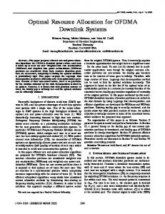
select the M particles to span the feasible space of the resource allocation, as much as possible. Figure 1 illustrates a minuscule project of only n = 2 activities, M = 5 particles, and the forces on particle #3. Each particle in this ´ ³ (m) (m) space is defined by its two dimensions, x(m) = x1 , x2 , for m = 1, · · · , 5. The “charge” of each particle is a measure of the value of the objective function 4
u x(4) Feasible square of the allocations
Resultant Force F(3) x(5)
Each X(k) = (x1(k), x2(k)) la = l for all a and ua = u for all a
F(3,5)
x(2)
We assume that v(3) < v(1), v(5), therefore repulsed by them But v(3) > v(2), v(4), therefore attracted to them
F(3,2)
F(3,1) x(3)
x(1)
F(3,5)
l
u
Figure 1: Forces on particle #3 ¢ ¡ at that point, which is denoted by v x(m) , m = 1, · · · , M . This value is determined through Monte Carlo sampling of the vector of work content (wa )a∈A
which, together with the allocation x(m) , determine the “resource cost” as well (m)
as the time of project completion, denoted by tP path calculations. Knowledge of
(m) tP
through standard critical
enables one to determine the penalty for
tardiness beyond the specified project due date T. We define vmin as the minimal value among all M points, n ³ ´o vmin = min v x(m) . m
It is important, for stability reasons, to “normalize” and “scale” these values, which result in the charge q (m) at point x(m) . This charge is evaluated as follows, " # v(x(m) ) − vmin (m) q = exp −n × PM £ ¤ , m = 1, 2, ..., M. (k) ) − v min k=1 v(x 5
Observe that a large v(x(m) ) results in a small q (m) , and conversely, a small v(x(m) ) results in a large q (m) . Indeed, at vmin the charge is 1, the maximum. The charge q (j) of particle j determines the force of attraction or repulsion between particle j and the other particles. For each pair of particles x(j) and ¢ ¡ ¢ ¡ x(k) suppose that v x(j) < v x(k) , which implies that q (j) > q (k) . Then particle x(k) is “attracted” to particle x(j) by a force given by # " ´ ³ q (j) q (k) (j) (k) F (j, k) = x − x ×° ° , ∀ j, k, °x(j) − x(k) °2
(2)
and particle x(j) is “repulsed” by particle x(k) by a force of the same magnitude in the opposite direction. The direction of the attraction/repulsion force is along the line between the two particles with the arrow pointing from x(k) to x(j) for particle k and the reverse for particle j (i.e., along the same line away form k ). The (vector) resultant force F (m) on each particle m is calculated by conventional methods to yield the magnitude of the force and its direction of movement; see Fig.1. The force F (m) is then normalized to yield, F (m) = vector sum (F (j, m)) , j 6= m, m = 1, · · · , M. This procedure is repeated for each particle x(m) , m = 1, · · · , M to yield the
values of the forces at all M particles in the population. Each particle x(m) is then moved in the specified direction by a random step given by, 0 (m) (m) x(m ) ← x(m) + β · (RN G) · Fnorm
β ∈ (0, 1) , in which β is selected randomly and (RN G)(m) is the “range" of movement of the particle; a measure of the allowed feasible movement toward the upper or lower bounds, depending on the movement of the point. The movement of the particles continues X (1) → X (2) → · · · → X (I) until the stopping condition is satisfied (with I = 25n). The allocation that yielded vmin when iteration is halted is selected as the “optimal” allocation. For each replication (R) of the experiment, a set of K = 100 W ’s is generated and stays fixed thereafter. For each of the M particles consecutively 6
generated during the EMA iterative process, the corresponding value of the objective function is evaluated, for each of the W ’s generated. In other words, we evaluate the value of the objective function for each of the particles, for each of the 100 W ’s. The value of the particle is based on the average of the 100 PK values, v (m) = k=1 v(k) /K. It is these values that are used in the EMA to
decide on the forces acting on the particle. Finally, when we stop the movement
of the particles (i.e., after 25n movements) we have one particle vmin which average value (over the 100 W ’s) is minimal. And to gain some idea about the variability of vmin the whole experiment (with M particles and different K samples of the work content) was replicated R times. In our experimentation we took R = 4. The minimum over these four replications is the value we quote in Table 1.
4
Experimental Layout and Computational Results
The program outlined above was implemented in Matlab on a set of fourteen projects that ranged in size from 3 to 76 activities. The networks under study can be seen in the internet1 , or requested by e-mail from the lead author2 . The results obtained (on a Pentium IV, 3 GHz, 1 GB RAM) are in the same web pages cited, and are summarized in Table 1. In all networks, the allocation to any activity, xa , is constrained to be in the interval [0.50, 1.50]. The resource cost proportionality constant ka is normalized at 1, the same for all activities. The tardiness penalty cL is as given in Table 1. The “PERT Expected Value” is the length of the so-called “critical path” following the PERT model. This, together with the due time T give an idea about the “tightness” of the imposed due time (recall that the PERT expected duration is an underestimate of the exact expected duration), and was maintained in the range (T /E (P ERT )) ∈ [1.03, 1.09] throughout. The value of K was fixed at 100 for all experiments; that is, 100 work content samples were generated for each iteration in each experiment. The 1 www.dps.uminho.pt/pessoais/anabelat
(Topic: research).
2
[email protected].
7
experiment was repeated R = 4 times. The values quoted in Table 1 are the best in the four replications, as explained above. The restriction to 2 and 3 discrete points in the DP approach was necessary to keep the computing time within reasonable limits. Still, DP failed to reach a solution for networks of n ≥ 24 within 48 hrs. This is where the superiority of the EMA is manifested. In fact, the EMA gives a better “best value" than DP in several instances of even small networks. The cause lies in the discretization required by the DP approach, which clouds the assertion of optimality of its results.
PERT
DP
DP
DP
EMA
EMA
Net
n
Dur’n
T
cL
Points
Best Cost
DP Time
Best Cost
Time
1
3
15
16
2
3
43.32
0.1 sec
36.57
14.0 sec
2
5
115
120
8
3
304.62
1.0 sec
277.53
32.4 sec
3
7
62.9
66
5
3
209.94
3.0 sec
207.33
1.1 min
4
9
100
105
4
3
387.20
1.1 min
379.67
1.8 min
5
11
26.67
28
8
3
106.76
7.4 min
115.19
2.3 min
6
11
62.08
65
5
3
280.85
45.5 min
286.30
2.7 min
7
12
44.72
47
4
3
182.91
5.8 hr
183.19
3.5 min
8
14
35.5
37
3
2
116.49
31.9 min
122.67
4.2 min
9
14
178.57
188
6
2
645.39
6.5 hr
710.27
5.0 min
10
17
44.98
49
7
2
160.12
4.2 hr
137.53
7.5 min
11
18
106.11
110
10
2
339.07
30.2 hr
375.43
9.7 min
12
24
212.05
223
12
2
-
> 48hr
1212.00
18.5 min
13
38
143.99
151
5
2
-
> 48 hr
834.77
1.0 hr
14
76
115.01
121
4
2
-
> 48 hr
559.19
6.2 hr
Table 1. Experimental Results
5
Conclusions and Future Research
The results demonstrate: 1. The superiority of the EMA in value over the DP approach for many 8
networks. As stated before, this is due to the large “mesh” used in DP (only 3 points in the first seven networks and 2 points in the remaining (larger) seven networks). Finer mesh should yield better results, at the cost of (severely) increased computational burden. 2. The computational superiority of the EMA over DP for the larger networks by several orders of magnitude. 3. The advantage of the use of EMA with repeated experimentation. This advantage is twofold. First, it does provide an estimate of the expected cost of the project. Second, one can use the replication of the experiment R times for any given network to estimate the range of variation of the expected value. As an example, this was done with Net 5 in the above table. The results of the best values were as follows: 127.71, 115.19, 122.62, 132.06, for an average of 124.40 and variance ≈ (7.25)2 . The best average cost is 115.19 which corresponds to the allocation x∗ = (1.50, 1.50, 0.64, 1.38, 1.50, 1.45, 0.69, 1.47, 1.50, 1.50, 0.99) .
(3)
(Observe that 5 of the 11 activities were at the upper bound of resource allocation, which may hint at securing a smaller expected value if the resource capacity is increased — an important indication to management.) More importantly, assuming normality, one can ascertain that with probability of approximately 97.7% the optimal expected value of this project is larger than 109.90. To be sure, all four values lie above this value. Furthermore, by adopting the x∗ of (3) we are only 115.19 − 109.90 = 5.29 units away from the lower bound on cost, or less than 4.8%. 4. The assumption of exponential distribution of the work content was made for ease of discretization of the work content in the DP approach, and is central in the analysis of Markov activity networks. It is irrelevant to the EMA approach which would accept any distribution, since the random variables enter the approach only via the sampled W ’s.
9
Matlab is not the ideal language for industrial applications, and we are confident that if the logic of EMA is coded in another language such as C or C ++ by an expert programmer the time required to reach a solution will improve by at least one order of magnitude. It is important to achieve efficient codes because, while it is true that the result given by EMA is the optimal vector x∗ , this is a static policy which may be, and in all probability shall be, modified dynamically later. To change the picture from a static optimum to a dynamic one, we propose that only the allocations to the activities along the cutset at the start of the project are implemented. The resource allocation to other activities should await the progress of the project. As the project progresses some of the activities in the initial cutset will be completed and the status of the project will change. At which time the new information is incorporated into the model and the EMA is re-run. This process continues until the project is completed. Therefore, in the span of time in which the project is “alive" the EMA procedure may be run several times, each on a different network, possibly with updated values on the distributions. The networks get smaller and smaller as activities are completed, and consequently the time required to run EMA also gets smaller. Apart from improved programming of the logic of the EMA, our research is currently directed towards the improvement of the performance of the EMA itself, possibly through improved local search, improved dynamic update of the step size, and improved layout of the particles in the feasible space.
10
References [1] S.I. Birbil, and S-C. Fang, An Electromagnetism-Like Mechanism for global optimization, Journal of Global Optimization 25, 2003, pp. 263—282. [2] A.P. Tereso, M.M. Araújo, and S.E. Elmaghraby, Adaptive Resource Allocation in Multimodal Activity Networks, International Journal of Production Economics 92, 2004, pp. 1-10 . [3] A.P. Tereso, M.M. Araújo, and S.E. Elmaghraby, Experimental Results of an Adaptive Resource Allocation Technique to Stochastic Multimodal Projects, Research Report, Universidade do Minho, Guimarães, Portugal, 2003 (Submitted for publication). [4] A.P. Tereso, M.M. Araújo, and S.E. Elmaghraby, Basic Approximations to an Adaptive Resource Allocation Technique to Stochastic Multimodal Projects. Research Report, Universidade do Minho, Guimarães, Portugal, 2003 (Submitted for publication).
11