Optimal Testing Effort Control for Modular Software System ...

An International Journal of Optimization and Control: Theories & Applications Vol.2, No.2, pp.129-137 (2012) © IJOCTA ISSN: 2146-0957 eISSN: 2146-5703 http://www.ijocta.com

Optimal Testing Effort Control for Modular Software System Incorporating the Concept of Independent and Dependent Faults: A Control Theoretic Approach Kuldeep CHAUDHARY a and P. C. JHA a a

Department of Operational Research,University of Delhi - India Email: [email protected] Email: [email protected] (Received August 01, 2011; in final form June 02, 2012)

Abstract. In this paper, we discuss modular software system for Software Reliability Growth Models using testing effort and study the optimal testing effort intensity for each module. The main goal is to minimize the cost of software development when budget constraint on testing expenditure is given. We discuss the evolution of faults removal dynamics in incorporating the idea of leading /independent and dependent faults in modular software system under the assumption that testing of each of the modulus is done independently. The problem is formulated as an optimal control problem and the solution to the proposed problem has been obtained by using Pontryagin Maximum Principle. Keywords: Software reliability growth models; Testing resource allocation; Modular software system; Pontryagin maximum principle; Testing-effort expenditure. AMS subject classifications: 90B99, 68M99, 49N90, 97M10.

1. Introduction The software development industry has grown dramatically in scope, complexity and pervasiveness over the last few decades at an unprecedented pace. The Internet has practically transformed the world into a big computer network, where communication, information and business are constantly taking place on-line. Most industries are highly dependent on computers for their basic day-to-day functioning. Safe and reliable software operation is a significant requirement for many types of systems. Aircraft and air traffic control, medical devices, nuclear safety, petrochemical control, high speed rail, financial systems, automated manufacturing, military and nautical systems, aeronautics, space missions and appliance-type applications such as automobiles, washing machines, temperature control and telephony are highly computerized.

The cost and consequences of these systems failure can range from mildly annoying to catastrophic, with serious injury occurring or lives lost. As software assumes more responsibility for providing functionality and control in these systems, it becomes more complex and significant to the overall system performance and dependability. The software reliability assessment is important to evaluate and predict the reliability and performance of a software system. The models applicable to the assessment of software reliability are called Software Reliability Growth Models (SRGMs). Starting from the late sixties, in the approximately past 40 years a vast literature of software reliability models has been developed. Extensive research exists in modeling the failure detection and fault removal phenomenon by an Non-homogenuous poisson process (NHPP) [1,2,3]. These models have been widely studied

Corresponding Author. Email: [email protected] 129

130

K.Chaudhary, P.C. Jha / Vol.2, No.2, pp.129-137 (2012) © IJOCTA

and applied on real software projects. Many concepts of software reliability modeling have been developed and models are proposed considering the various dynamic aspects of the software testing and debugging. Most of these models assume a perfect debugging environment. This means whenever an attempt is made to remove a detected fault it is removed perfectly and no new faults are generated. The earliest model in this category was due to Goel and Okumoto [4]. Some other models in this category are Yamada et al. [5]; Ohba [6, 7]; Yamada and Osaki [8]; Bittanti et al. [9] and Kapur and Garg [10] etc. Testing efforts plays a very crucial role on the testing progress. For example, at any instance of time during the testing phase testing can be made more rigorous through the additional testing efforts. A model that accommodates the effect of testing effort on the reliability growth more often proves to be more useful in the later phases of the testing as it can be used to determine the amount of additional efforts required to reach a specified reliability objective. Most of these earlier SRGMs use execution time as the unit of fault detection/removal period and either assume that the consumption rate of testing resources is constant or do not explicitly consider the testing effort and its effectiveness. A testing effort function describes the distribution or consumption pattern of testing resources (CPU time, manpower, etc) during the testing period. Putnam [11]; Yamada et al. [12, 13, 14]; Bokhari and Ahmad, [15]; Kapur et al. [16, 17]; Kuo et al. [18] and Huang et al. [19, 20, 21], proposed SRGMs describing the relationship among the testing time (calendar time), testing-effort expenditure and the number of software faults detected. Most existing SRGMs belong to exponential-type models. Kapur et al. [17] and Huang et al. [19, 20, 21] proposed S-shaped testing effort dependent SRGM based on Yamada delayed S-shaped model which also describe the leaning phenomenon of the testing team. The optimal control theory is a branch of mathematics developed to find optimal ways to control a dynamic system. Most early developments are reported in engineering literature. Optimal control problems with state variable inequality constraints arise frequently not only in Mechanics and aerospace engineering but also in area of management sciences and economics [22, 23, 24, 25, 26, 27]. In the present paper, we applied optimal control theory to solve

a general and important problem related to modular software system for SRGMs using testing effort as a control variable. In this paper, we discuss modular software system for SRGM using testing effort and how to allocate optimal testing effort to each module such that the total amount of testing effort expenditure is fixed. Here we assume that software firm wants to plan the testing process for the different modules with the objective to minimize the total software testing cost. Testing of each modules is done independently. We formulate an optimal control theory problem for modular software system and study the optimal testing effort expenditure rate towards each module. And, we apply Maximum Principle to solve testing effort allocation problem in modular software system. We organized the paper as follows. In Section 2, we discuss the evolution of faults removal dynamics in modular software system under the assumption that testing of each modules is done independently and practitioner may choose independently the testing effort intensity directed to each different module. The problem is discussed and solved using Pontryagin’s Maximum principle with Particular cases in Section 3.

2. Model Formulation Testing is an important stage of Software Development Life Cycle as it provides the measure of software reliability and assists to judge the performance, safety, fault tolerance or security of the software. As most software systems are modular, it is of great importance for the management to allocate the limited testing effort recourses among the software modules in an optimal way. Testing effort can be measured by the manpower, the number of test cases, the number of CPU hours etc. There exist a number of successful S-shaped models in literature of the software reliability but we are mainly concerned here with the Kapur and Garg model [10] due to its simplicity and capability to study the failure growth rate of software. It has been observed that during testing, the team can remove some faults in the software, without these faults causing any failures. Fault which is removed consequent to failure is known as a leading fault. While removing the leading faults, some other faults are removed which may have caused failure. These faults are known as dependent faults.

Optimal Testing Effort Control for Modular Software System …

We begin our analysis by describing a model for modular software system with a very few number of assumptions [19, 1]. Here are the modeling assumptions: 1) The fault removal process follows the Non Homogenous Possion Process (NHPP). 2) The software system is composed of N independent modules that are tested independently. 3) The total amount of testing resources expenditure available for the module testing processes is fixed and denoted by W . 4) The system manager has to allocate the total testing resources W to each software module to minimize the number of faults remaining in the system during the testing period. 5) If any of the software modules is faulty, the whole software system fails. 6) The detection of the error causing failure also results in detection of the remaining errors without those errors causing any failure. With these assumptions, the number of faults detected by the current testing effort expenditure is proportional to the number of remaining faults. The evolution of fault removal dynamics for each modules can be described by the following differential equation:

m t    dmi (t )  wi (t )  pi  ai  mi  t    qi i ai  mi  t     dt ai  

mi (0)  0 ,  i  1to n

(1) Where, mi(t) is the expected mean number of faults detected in time (0, t) in ith module, ai is initial number of faults in ith module in the software before start of testing phase, pi is the fault detection rate, qi is the fault detection rate of additional faults and wi is current testing effort expenditure rate in the time interval (0,t] for ith modules. W (t ) is the allocated amount of

i

testing resources expenditure for ith module and

d W (t )  w (t ) . i dt i We can evaluate the total software cost by using cost criterion, the cost of testing-effort expenditures during software development and testing phase, and the cost of correcting errors before and after release [28]. Therefore, the total software cost for each module as follows

131

C1i ( wi ) mi T   C2i ( wi )  mi     mi T      (2) T C t       C w t dt i 1   3i  i   0   n

Where, C1i is the cost of testing effort ( wi ) utilized for correcting an error during testing for ith module, C2i is the cost of testing effort ( wi ) utilized for correcting an error in operational use for ith module  C2i  C1i  and C3i is the cost of testing per unit testing effort expenditure for ith module. Note that the expected cost of fixing a fault after release is usually higher than the expected cost of fixing a fault during testing. As t  , the expected number of fault to be detected is mi    and it should be finite value i.e. mi     Ai =constant, then the equation (2) can be re-write as follow: C1i ( wi ) mi T   C2i ( wi )  Ai  mi T    n   T C t      i 1  C3i wi (t ) dt   0   (3) Here, optimization problem is how to allocate optimal testing effort to each module such that the total amount of testing effort expenditure for all modules is fixed. We formulate an optimal control problem to allocate an optimal amount of testing effort to each modules to minimize the total software testing cost. The problem consisting of choosing the control variable wi (t ) such that it minimizes the total testing cost at time t, with the requirement that there are N modules in system. Let T is the release time of software product. Now the objective can be written as T  n C ( w ) m t   1i i i    min J       dt wi ( t )    C ( w ) A  m t  C w     0  i 1  2 i i i i 3 i i    (4) subject to (1) and the testing resources expenditure constraints for all modules

 n  wi dt  W 0   i 1 

T

(5)

Constarint (5) corresponds to the common testing effort allocation resourse capacity that is allocated among all the modules. This is the only

K.Chaudhary, P.C. Jha / Vol.2, No.2, pp.129-137 (2012) © IJOCTA

132

constraint that is coupling the modules and prevents us from simply solving n times a singlemodule problem. Therefore, the modules dependent testing problem is equivalent to determine the minimal cost for all modulus and testing effort rate wi (t )  0 and associated fault detection rate

 n  C2i ( wi )  C1i ( wi )  mi  t    max J       dt  wi ( t )   0  i 1  C2i ( wi ) Ai  C3i wi s.t.

mi (t ) satisfy the system equation (1).

mi (0)  0

The optimal control formulation can be written as:

 n  wi dt  W 0   i 1 

T

(P1)

To solve the above optimal control theory problem (P1), we have introduced a new state variable B(t) into the problem such that the integral constraint can be replaced by a condition in terms of B(t). 0

n i 1

wi   d Where, the

upper limit of integration is the variable t , not the terminal time T . The derivative of this n variables is B  t   i 1 wi  t  (Equation of motion for B(t)) . And the terminal values of B(t) in the testing period are

B(0)  0 and B T   

T

0



n i 1

n

Thus, we have an optimal control problem with n control variable(wi(t)) and n+1 state variable (mi(t), B(t)) for all modules. To solve the , we define the Hamiltonian as n  C ( w )  C ( w )   (t ) m (t )   i   n   2i i 1i i i H      (t )   wi   C ( w ) A  C w ( t ) i 1   i 1   2i i i 3i i 

(7) A simple interpretation of the Hamiltonian is that it represents the sum of current cost  C2i (wi )  C1i (wi )  mi t  and future cost

3. Solution and Results of Proposed Optimal Control Problem



B  t    i 1 wi  t  , B (0)  0, B T    W (P2)

 pi  ai  mi  t      dmi (t )  wi (t )  mi  t   , mi (0)  0 dt   qi a  ai  mi  t    i  

t

  m t   dmi (t )  wi (t )   pi  qi i   ai  mi  t      dt ai   

ui0  wi  t   ui , 0  ui0  1, 0  ui  1, ui0  ui

 n  C2i ( wi )  C1i ( wi )  mi  t    max J       dt  C ( w ) A  C w wi ( t ) 0  i 1  2i i i 3i i   s.t. T

Let us define B  t   

T

wi ( ) d  W (6)

Using new state variable with terminal conditions (6), we can restate optimal control problem (P1) as follow:

i (t ) mi  t  . Assuming the existence of an optimal control solution, the maximum principle provides the necessary optimality conditions [29]. There exists a piecewise continuously differentiable function λi(t) and µ(t) for all tϵ[0,T]. Where λi(t) and µ(t) are known as adjiont variables and the value of λi(t) and µ(t) at time t describe the marginal valuation of state variables mi(t) and B(t) at time t respectively (or λi(t) stands for future cost incurred as one more fault introduced in the system at time t and µ(t) is the future cost of testing per unit testing effort expenditure at time t ). It describes the similar behavior in optimal control theory as dual variable have in non linear programming. The following necessary optimality conditions holds for an optimal solution:

Optimal Testing Effort Control for Modular Software System …

 H *  w t  0  i   d  (t ) H   , i (T )  0  i mi  t   dt  d  (t ) H    , B  t   dt    T   0, B T   W  0,  T   B T   W   0

(8)

Where  T   0 , B T   W  0 ,

 T   B T   W   0 are transversality condition for B(t). The Hamiltonian is independent of B(t), we have   H / B  0    t   constant . It is

clear that the multiplier associated with any integral constraint is constant over time irrespective of their nature (i.e. whether equality or inequality). From the optimality conditions, we get the testing * effort rate wi  t  for each module.    C2i  Ai     C3i    t    w i     1   wi*  t     p  q mi  t   a  m t    C2i C1i     i i  i i     ai        wi wi      C2i ( wi )  C1i ( wi )  i (t )  

  m t   dmi (t )  wi (t )   pi  qi i ai  mi  t        dt ai   

(10) d i m H *   t       C2i  C1i  i  i dt mi mi

(11)

t

   

0

testing effort towards ith module. The above equation takes the form

   1  e  pi  qi  Wi (t )   mi (t )  ai   1  qi e pi  qi  Wi (t )    pi   (12) Equation (12) gives the optimal number of faults detected in time (0, t) in ith module. Integrating equation(11) with condition λi(T)=0, we have the future cost of removing one more fault can be given as  T  m   i  t   h(T ) exp     i  dt    C2i (wi (t )  C1i (wi (t )   t  mi   Where, h(T )   C2i (wi (T )  C1i (wi (T ) 

Particular Cases: In the next section, we examine the behaviour of the proposed optimal control problem by changing the correcting costs.

In this section, we assume that the costs are linear function of testing effort i.e. C1i ( wi )  C1i wi

As mi (t )  ai , value of testing effort rate increasing and becomes very large. From equations (1), (8) and (9), the adjoint and state variables respectively can be defined as

  pi  qi   wi ( ) d  0 1 e   mi (t )  ai t   pi  qi   wi ( ) d 0 1  ( q / p ) e i i 

t

Define Wi  (t )   wi ( ) d as the cumulative

3.1. When the costs are linear function of testing effort

(9)

with terminal conditions mi(0)=0 and λi(T)=0. The solution of the equation(10) is

133

and C2i ( wi )  C2i wi . Where C2i andC1i constant values. Now Hamiltonian can be written as

are

n   C  C  w   (t )  m (t )   n  1i i i i  2i  H      (t )   wi  i 1    C2 i Ai  C3i  wi i  1     

(13) From the optimality conditions, we have optimal * value of testing effort rate wi  t  for each module. The optimal testing effort for each module is      C3i    t   C2i A1    (t ) 1  wi*  t     i 2  C2i  C1i      mi  t    p  q a  m t         i i i i    a i      

(14) The optimal value of adjoint and state equations are    T  m   i  t    C2i  C1i   wi (T ) exp     i  dt   wi (t )     t  mi    

134

K.Chaudhary, P.C. Jha / Vol.2, No.2, pp.129-137 (2012) © IJOCTA

 t   pi  qi   wi ( ) d 0  1 e mi (t )  ai  t   1  qi e pi  qi  0 wi ( ) d  pi 

     

define the Hamiltonian as n  C  C   (t ) m (t )   i   n   2i 1i i H      (t )   wi  i 1   i 1  C2i Ai  C3i wi (t )  The

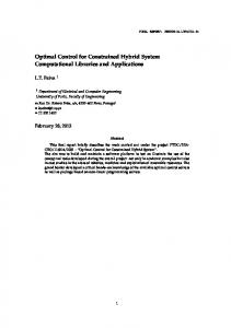
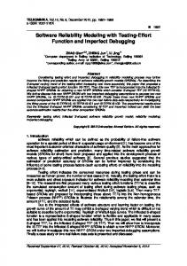
The physical interpretation of the above optimal policies for the testing effort allocation can be decribed as: Intially mi(t) increases due to S-shaped nature of fault detection function, then allocation path of testing effort expenditure will decrease. Later allocation path of testing effort expenditure will start increasing, when mi(t) slow down due to S-shapedness in fault detection rate.



(15) n i 1

C2i Ai

term in the

Hamiltonian

function is constant. Moreover, the fixed value



n i 1

C2i Ai can be omitted in the equation.

Since the Hamiltonian is linear in control variable, the maximum principle given the following condition for the optimal testing effort wi*  t  :

 ui0  wi*  t    Singular u  i

, if Di (t )  0 , if Di  t   0 i (16) , if Di  t   0

Here,

Di (t )   C2i  C1i   i  t 

mi  C3i    t   H wi wi

is the coefficient of wi in H and it is called the “switching function” and is illustrated in Fig.3. This type of optimal control is known as “bangbang” in the terminology of optimal control theory. However, interior control is possible on an arc along which Di  t   0 . Such an arc is Figure 1. Optimal path of fault detection.

known as a “singular arc”. More generally, the extremal arcs

H

wi

0



on which the matrix

H wi wi is singular arcs [27]. Now, the equation (16) can be written as

m  0 , if  C2i  C1i  i  i  C3i  i ui wi  * wi  t    Singular , if Di  t   0  m  ui , if  C2i  C1i  i  i  C3i   wi  (17) Figure 2. Optimal testing effort allocation policy.

3.2. When the costs are constant In this section, we assume that the costs C1i and

C2i are not directly dependent on testing effort rate i.e. C1i ( wi )  C1i and C2i ( wi )  C2i . Where C2i andC1i are constant values [20]. To solve the optimal control problem, we can

The interpretation of the optimal polices given by equation (17) can be described as follows: If the total cost of correcting an error is less than the unit testing cost, then all testing effort expenditure rate should be minimum for all modules. On the other hand, if total cost of correcting an error is greater than the unit testing cost, then all testing effort expenditure rate should be maximum for all modules.

Optimal Testing Effort Control for Modular Software System …

135

4. Conclusion D(t) >0 D(t)