fer problem is solved using the solution to the multiple-revolution Lambert problem. A solution procedure is proposed based on the study of an auxiliary transfer ...
JOURNAL OF GUIDANCE, CONTROL, AND DYNAMICS Vol. 26, No. 1, January–February 2003
Optimal Two-Impulse Rendezvous Using Multiple-Revolution Lambert Solutions Haijun Shen¤ and Panagiotis Tsiotras† Georgia Institute of Technology, Atlanta, Georgia 30332-0150 The minimum-¢V, xed-time, two-impulse rendezvous between two spacecraft orbiting along two coplanar unidirectional circular orbits (moving-target rendezvous) is studied. To reach this goal, the minimum-¢V, xed-time, two-impulse transfer problem between two xed points on two circular orbits is rst solved. This xed-endpoint transfer is related to the moving-target rendezvous problem by a simple transformation. The xed-endpoint transfer problem is solved using the solution to the multiple-revolution Lambert problem. A solution procedure is proposed based on the study of an auxiliary transfer problem. When this procedure is used, the minimum ¢V of the moving-target rendezvous problem without initial and terminal coasting periods is obtained for a range of separation angles and times of ight. Thus, a contour plot of the cost vs separation angle and transfer time is obtained. This contour plot, along with a sliding rule, facilitates the task of nding the optimal initial and terminal coasting periods and, hence, obtaining the globally optimal solution for the moving-target rendezvous problem. Numerical examples demonstrate the application of the methodology to multiple rendezvous of satellite constellations on circular orbits.
I
Introduction
orbits. He showed that allowing more than one revolution may reduce fuel consumption. However, Prussing does not identify which of the possible 2Nmax C 1 solutions provides the least cost. As a result, the minimum-cost solution is obtained only after calculating all 2Nmax C 1 candidates. In this paper, we provide an algorithm that quickly and ef ciently identi es the optimal (minimum1V ) solution without the need to calculate all 2Nmax C 1 transfer orbits. This paper is organized in the following manner: After the Introduction, the formulation of the minimum-1V , xed-time, xedendpoint orbital transfer problem is presented, then the auxiliary transfer problem is introduced and its solution is analyzed. The solution to the auxiliary transfer problem is then applied to the xed-endpoint transfer problem. Next, solutions to the movingtarget rendezvousproblem without initial and nal coasting periods are obtained for a range of separation angles and times of ight. The global optimal solution for the moving-target rendezvous problem can then be obtained by applying a sliding rule.6 As an application to the proposed methodology,in the last section of the paper we analyze rendezvousmaneuvers motivated by the problem of servicing satellites in a circular constellation.
N this paper, we are interested in nding the best two-impulse solutions for a class of rendezvous problems. Speci cally, we study the xed-time, two-impulse rendezvousproblem between two spacecraft. Both the chaser and the target spacecraft move on two coplanar circular orbits in the same direction. The motivation for investigatingsuch two-impulse xed-timerendezvousproblemsstems from our interest in solving multiple rendezvous problems between several vehicles in a satellite constellation. Clusters of satellites and satellite constellations (including formation ying schemes) promise to provide increased exibility, autonomy, reliability, and operabilitycomparedto traditionalsingle-spacecraftapproaches.1¡3 In many cases, the satellites in the constellation can be serviced either from a vehicle launched from Earth for that purpose or by other satellites in the same constellation.4 Such scenarios require a complete understanding of multiple orbital transfers between a number of satellites. Before being able to solve the multiple-rendezvous problem for a satellite constellation (which may include dozens or hundreds of satellites) it is imperative to have a complete characterization for the simplest case of an optimal rendezvous, namely, between two satellites in a circular orbit. As a matter of fact, as shown in this paper,even the simple case of prioritizingthe rendezvousmaneuvers between three satellites is not clear from the outset. The results of this paper, thus, lay the foundation for solving ef ciently optimal and suboptimal rendezvous strategies in a constellation with many satellites. In Ref. 5 a solution procedure is outlined for the multiplerevolution Lambert problem. It is shown that given two points and a speci ed time of ight long enough to allow Nmax revolutions for the chaser, there exist 2Nmax C 1 Keplerian orbits that pass through the given two points. With the use of the solutions to the multiplerevolution Lambert problem, Prussing5 studied the minimum-cost, xed-time transfer between two xed points on coplanar circular
Fixed-Time, Fixed-Endpoint Transfer Between Circular Orbits Given two points P1 and P2 in space, there are two elliptic orbits with the same semimajor axes that connect the two points, as shown in Fig. 1. In Fig. 1, F and F ¤ are the primary and secondary foci of the transfer orbits, r1 and r 2 are the radii from F to the points P1 and P2 , respectively, d is the length of the chord connecting P1 and P2 , and µ is the central angle between r1 and r 2 . The two orbits in Fig. 1 belong to two separate categories: the long-path transfer orbits and short-path transfer orbits. As seen in Fig. 1, for a long-path transfer orbit, F and F ¤ lie on opposite sides of the P1 P2 line segment, whereas for a short-path transfer orbit, F and F ¤ lie on the same side of the P1 P2 line segment. For a given transfer time t f , an N -revolution transfer orbit is an elliptic orbit passing through P1 and P2 , and the time of travel along the P1 P2 arc plus N complete revolutions is t f . An N -revolution transfer then is one where the chaser spacecraft moves along the elliptic transfer orbit for N complete revolutions plus the P1 P2 arc before meeting the target at P2 . In general, there is more than one elliptic orbit that passes through P1 and P2 for a given travel time t f , depending on the number of revolutionsallowed. These orbits are either long-path or short-path orbits with different semimajor axes. According to Lambert (see Ref. 7), the time of ight is a function only of the semimajor axis a, the sum of the radii r1 C r2 , and the
Received 15 November 2001; revision received 19 July 2002; accepted c 2002 by Haijun Shen and for publication 25 September 2002. Copyright ° Panagiotis Tsiotras. Published by the American Institute of Aeronautics and Astronautics, Inc., with permission. Copies of this paper may be made for personal or internal use, on condition that the copier pay the $10.00 per-copy fee to the Copyright Clearance Center, Inc., 222 Rosewood Drive, Danvers, MA 01923; include the code 0731-5090/03 $10.00 in correspondence with the CCC. ¤ Ph.D. Candidate, School of Aerospace Engineering; haijun shen@ ae.gatech.edu. Member AIAA. † Associate Professor, School of Aerospace Engineering; p.tsiotras@ ae.gatech.edu. Associate Fellow AIAA. 50
SHEN AND TSIOTRAS
51
Fig. 1 Orbital geometry for Lambert problem.
Example graph of tf vs a.
Fig. 2
chord length d. Lagrange’s formulation of the Lambert problem can be generalized to the multiple-revolutioncase as5 3 p ¹t f D a 2 [2N ¼ C ® ¡ ¯ ¡ .sin ® ¡ sin ¯/] (1) where ¹ is the gravitational parameter, N is the number of allowed revolutions, and ® and ¯ are de ned as follows: 1
sin.®=2/ D [s=.2a/] 2 ;
1
sin.¯=2/ D [.s ¡ d/=.2a/] 2
(2)
where s D .r 1 C r2 C d/=2. A geometric interpretation of the variables ® and ¯ can be found in Ref. 8.
In the following, canonicalunits are used in the calculations.That is, the reference circular orbit has radius r1 D 1 and period 1. Hence, ¹ D 4¼ 2 , and the velocity unit is the reference orbital speed divided by 2¼ . An example plot of t f vs the semimajor axis a is shown in Fig. 2. Figure 2 is drawn with the help of Eq. (1). N denotes the number of revolutions.The plot in Fig. 2 corresponds to the case where r1 D 1, r 2 D 2, and µ D 60 deg. For each N , two solution branches exist, an upper branch and a lower branch. The upper branch corresponds to a long path for µ · 180 deg, and a short path for µ ¸ 180 deg; the lower branch corresponds to a short path for µ · 180 deg, and a
52
SHEN AND TSIOTRAS
long path for µ ¸ 180 deg. For each N ¸ 1, there are two semimajor axes correspondingto the same t f , and they de ne two N -revolution transferorbits (short-pathand long-pathorbits).However,for N D 0, the lower branchis monotonicallydecreasingand so there is only one semimajor axis that correspondsto the same t f (either for the shortpath orbit or for the long-path orbit). Therefore, for a given t f , there are 2N max C 1 solutions for the multirevolution Lambert problem, where N max is the maximum number of allowed revolutions. For example, in Fig. 2, it is shown that for a time of ight of t f D 7:6 we have N max D 5. It is clear that there is a total of 11 semimajor axes that determine 11 different transfer orbits connecting P1 and P2 . A minimum-energyKeplerian orbit always exists connectingtwo given xed points in space.7 The semimajor axis of this minimum energy orbit is given by am D s=2. This is the minimum semimajor axis shown in Fig. 2. (This is the same for all branches.) The travel time corresponding to an N -revolution transfer orbit with semimajor axis am is denoted by tm ` , ` D 0; 1; : : : ; Nmax . A procedure for determining N max and solving for all 2Nmax C 1 transfer orbits for a given t f is provided in Ref. 5. Next, we consider the case where the two endpoints P1 and P2 lie on two coplanar unidirectional circular orbits. The objective is to nd the minimum-1V transferorbit for a chaser at P1 to rendezvous with a target at P2 in a given time of ight t f . Both the chaser and the target are moving along the two circularorbits before the rendezvous maneuver, and P2 is the location where the rendezvous takes place. This scenario is also shown in Fig. 1. For ease of reference we henceforth refer to this problem as the xed-time, xed-endpoint transfer problem. In the following, “cost” and 1V will be used interchangeably. Prussing5 has listed and compared the minimum costs for various cases of ratios of orbital radii and central angles. He is interestedin the questionof whether the long-pathor the shortpath transfer orbit renders the minimum cost. He also studies the optimal number of revolutions corresponding to the minimum-cost solution. In Ref. 5, it is shown that there are no clear patterns to facilitate the answer to these two questions. Therefore, a minimumcost transfer orbit is determined after all of the 2Nmax C 1 solutions have been calculated and compared. In the following sections, an auxiliary orbital transfer problem is introduced. This problem is slightly different from the formulation of the original xed-time, xed-endpoint transfer problem in the sense that the transfer time in the auxiliary transfer problem is free. It will be shown in the sequel that the solution to this auxiliary transfer problem greatly facilitates the solution to the underlying xed-time, xed-endpoint transfer problem. Indeed, at most two (instead of all 2Nmax C 1) solutions need to be computed to yield the minimum cost.
Auxiliary Transfer Problem The auxiliary transfer problem also seeks the two-impulse, minimum-cost transfer between any two points P1 and P2 in two coplanar circular orbits. However, unlike the xed-time, xedendpoint transfer problem, in the auxiliary transfer problem, the time of ight is free. The main purpose of the auxiliary transfer problem is to study the relation between 1V and the semimajor axis. An explicit expression of the 1V needed to transfer from P1 to P2 along a Keplerian orbit can be obtained from classical orbital mechanics, as follows9 : (3)
1V D 1V1 C 1V2
where 1V1 and 1V2 are the costs incurred at points P1 and P2 . They are given by 1Vi D
p
vi2 C vic2 ¡ 2vi vic cos Ái ;
i D 1; 2
(4)
where v1 and v2 are the orbital speeds at points P1 and P2 on the transfer orbit, v1c and v2c are the orbital speeds on the two circular orbits, and Á1 and Á2 are the elevation angles, that is, the angles at P1 and P2 between the velocities on the circular orbits and the velocities on the transfer orbit. Note that allowing for multiple revolutions does not change the 1V . However, the more the number of revolutions the longer
the transfer time will be. As a result, as shown in Fig. 2, there are two transfer orbits passing through P1 and P2 that have the same semimajor axis. One is the long-pathtransfer orbit, and the other the short-pathtransfer orbit. These two transfer orbits correspondto different times of travel. It is shown in the Appendix that the cost 1V for both the long-path and the short-path solutions of the auxiliary orbital transfer problem are a function of only the semimajor axis of the transfer orbit. However, the analytical relationship between a and 1V is rather complicated. Nevertheless, numerical results suggest a great deal of insight. To this end, we have plotted in Fig. 3 the relationship of 1V vs a for the cases where r1 D r 2 and r2 D 2r1 . In both cases µ D 120 deg. Extensive numerical studies show that the plots of 1V vs a for other combinationsof r1 , r2 , and µ have similar characteristicsas in Fig. 3. Thus, Fig. 3 will be used to induce salient properties of the solution. From Fig. 3, it is evident that there is a unique semimajor axis that corresponds to the minimum 1V . Let this be denoted by amin . The elliptic Keplerian transfer orbit with semimajor axis amin is the solution to the auxiliarytransfer problem. Interestingly,this transfer orbit is always a short-pathtransfer orbit. For the case where r1 D r 2 , we have that amin D r 1 D r2 , and, hence, the total 1V D 0. Figure 3 shows that amin is not a stationary point for 1V . This can also be veri ed that d.1V /=da does not exist at amin D r1 D r2 because in this case the eccentricity is zero. However, for the case r1 6D r 2 , Fig. 3 shows that amin is a stationary point for 1V . Hence, amin can be calculated by setting d.1V /=da D 0. Numerical schemes such as the Newton–Raphson algorithm or the bisection method can be used to compute amin . Detailed expressions for 1V and d.1V /=da can be found in the Appendix. As shown in Fig. 3, for a given semimajor axis,followingthe longpath transfer orbit always costs more than following the short-path transfer orbit. The cost associated with a long-path transfer orbit is monotonically increasing with a. For a short-path transfer orbit, however, the cost increases if the semimajor axis a is greater than amin and decreases if the semimajor axis is less than amin . Caution has to be exercised because it is not true that any long-path orbit always results in a larger cost than any short-pathorbit. For example, as seen in Fig. 3, a short-path transfer orbit with a large semimajor axis could be more costly than a long-path transfer orbit with a smaller semimajor axis.
Solution to the Fixed-Time, Fixed-Endpoint Transfer Problem Based on the observations made earlier about the characteristics of 1V with respect to a for the auxiliary transfer problem, the computations required for the minimum-1V solution for a xed-time, xed-endpointtransfer problem can be signi cantly reduced.This is especially true for cases with large times of travel that allow a large number of revolutions.As a result, in some cases, the minimum-1V solution is readily chosen by inspection; in other cases, only two of the 2N max C 1 solutions need to be calculated and compared to obtain the minimum-1V transfer orbit. Recall that given a xed-time, xed-endpoint transfer problem with transfer time t f , there are 2Nmax C 1 solution candidates, that is, there are 2Nmax C 1 semimajor axes corresponding to the same time of ight on the plot of t f vs a (Fig. 2). Each of these 2Nmax C 1 semimajor axes corresponds to an elliptic Keplerian transfer orbit. The semimajor axis that corresponds to the minimum-1V transfer orbit can be chosen by applying the observations made earlier about the auxiliary transfer problem to these 2Nmax C 1 semimajor axes. In the following, we present a solution procedure to achieve this goal. This will be demonstrated on the plot of t f vs a for a case µ · 180 deg. The case when µ > 180 deg can be treated similarly and is discussed brie y at the end of this section. We need to calculate the times of transfer t N ` and t N s from P1 to P2 along the long-pathand short-pathtransferorbits with semimajor axis amin with N revolutions,where N D 0; 1; : : : ; N max . This calculation can be done in a straightforward manner using Eq. (1). In the sequel, the subscript ` stands for the long-path and the subscript s stands for the short-path transfer orbit. Figure 4 shows, for instance, the values of t N s and t N ` for N D 4.
SHEN AND TSIOTRAS
53
a)
b) Fig. 3
Fig. 4
¢V vs a: a) r1 = r2 and b) r1 =/ r2 .
Case 2, tNs < – tf < – tN` and N =/ Nmax .
According to the comparison between t f and t N ` and t N s , .N D 0; 1; : : : ; Nmax /, there are four cases to consider. 1) If N max D 0, no revolution is allowed (case 1). Clearly, there is only one solution candidate, which is either a long-path or a shortpath solution. Thus, this is the optimal solution. For cases 2, 3, and 4, we assume that N max ¸ 1. 2) If t N s · t f · t N ` and N 6D Nmax , then amin is between the semimajor axes of the long-path transfer orbit and the short-path transfer orbit with N < Nmax revolutions (case 2). This is shown in Fig. 4. Recall that any short-path transfer orbit with a · amin costs less
than any long-path transfer orbit. Thus, the optimal solution is a short-path transfer orbit. In addition, for short-path transfer orbits, 1V monotonically decreases for a · amin and monotonically increases for a ¸ amin . Therefore, either the short-path N -revolution orbit (point R in Fig. 4) or the short path (N C 1)-revolution orbit (point L in Fig. 4) provides the minimum cost. However, there is no a priori knowledge regarding whether the former or the latter is the minimum-cost solution. Thus, both transfer orbits correspondingto points R and L in Fig. 4 need to be calculated. The one with the smaller cost is the optimal transfer orbit. A special subcase occurs
54
SHEN AND TSIOTRAS
Fig. 5
Subcase 3a, tNmax s < – tf < – tNmax ` and tf > – tmN max .
Fig. 6 Subcase 3b, tNmax s < – tf < – tNmax ` and tminNmax < – tf < – tmN max .
when N D 0. In this case, the short-path one-revolution orbit with a < amin provides the minimum cost because there is no short-path solution for a ¸ amin . 3) Case 3, when t N s · t f · t N ` and N D N max , is complicated by the fact that the short-path branch for N ¸ 1 is not monotonically increasing. Instead, t f has a stationary point. Let us denote by tmin N the value of the time of travel at this stationary point and by amin N the correspondingsemimajor axis. There are two subcases to consider. a) Case 3a, when t f ¸ tm Nmax , is shown in Fig. 5. Following a similar argument as in case 2, only two solutions need to be
calculated. These are the long-path and the short-path orbits corresponding to N D N max (points L and R in Fig. 5). The smaller of the two renders the minimum-cost transfer orbit. b) Figure 6 shows case 3b, when tmin Nmax · t f · tm Nmax . The two short-path N max -revolution solutions (points L and R in Fig. 6) need to be calculated and compared. The smaller one renders the minimum-cost transfer orbit. 4) In case 4, t N ` · t f · t.N C 1/s , that is, amin is between the semimajor axis of the N -revolutionlong-pathtransfer orbit and the semimajor axis of the (N C 1)-revolutionshort-path transfer orbit. There are three subcases to consider.
SHEN AND TSIOTRAS
55
Fig. 7 Case 4a, tf > – tNmax` .
Fig. 8
Case 4b, t(Nmax ¡ 1)` < – tf < – tNmax s and am < – amin < – aminNmax .
a) In subcase 4a, t f ¸ t Nmax ` , that is, amin is less than the least semimajor axis candidate, as seen in Fig. 7. In this case, only two candidates need to be calculated (points L and R in Fig. 7). These are the N max -revolutionlong- and short-path transfer orbits. The one with the smaller 1V is the optimal solution. b) In subcase 4b, t.Nmax ¡ 1/` · t f · t Nmax s but am · amin · amin Nmax . This is shown in Fig. 8. In this case, amin is less than the least semimajor axis candidate. Because the closest semimajor
axis candidate corresponds to a short-path transfer orbit, it follows that this transfer orbit is the minimum-1V solution. c) Subcase 4c includes all remaining cases under the condition of case 4. The situation is shown in Fig. 9. The (N C 1)revolution short-path transfer orbit requires less 1V than any other solution with a · amin and any long-path transfer orbit. Similarly, the N -revolutionshort-path transfer orbit requires less 1V than any other short-path transfer orbit with a ¸ amin . Therefore, as before,
56
SHEN AND TSIOTRAS
Fig. 9
Case 4c, tN` < – tf < – t (N + 1)) s , excluding subcases 4a and 4b.
only two solutions need to be calculated and compared. These are the N -revolution and N C 1 revolution short-path solutions (points L and R in Fig. 9). The one with the smaller 1V represents the minimum-1V transfer orbit. If N D 0, the one-revolutionshort-path transfer orbit provides the minimum 1V . The described procedure allows one to determine the minimum1V transfer orbits for xed-time, xed-endpoint transfer problems where µ · 180 deg. However, similar rules can be obtainedfor cases where µ > 180 deg. In such cases, the lower branch correspondsto a long-pathtransfer orbit and the upper branch correspondsto a shortpath transfer orbit. For brevity, we do not elaborate any further on the case µ > 180 deg; the interested reader should be able to derive the corresponding results vis-`a-vis the case µ · 180 deg.
Minimum-¢V , Fixed-Time, Two-Impulse Rendezvous Between Circular Orbits
Problem Description
So far we have presented a procedure for obtaining the xedtime, minimum-1V transfer orbit between two xed points on two coplanar unidirectional circular orbits. In this section, we apply this procedure to nd solutions to the moving-target rendezvous problem.To this end, considertwo space vehicles(denotedby s1 and s2 ) in two coplanar circular orbits moving in the same direction. Vehicle s1 is in the lower orbit, and s2 is in the higher orbit. The initial separation angle µ0 from s1 to s2 is given. The objective is to nd the minimum-1V , two-impulse trajectory for s1 to rendezvous with s2 in a given time t f . Although s2 initially leads s1 by the angle µ0 , the central angle measured from s1 to the location where the rendezvous is supposed to take place is µ D µ0 C t f !2
(5)
where !2 is the orbital frequency of the outer orbit. This is because s2 moves along the outer circular orbit during the maneuver. Essentially, once µ is known, that is, the projected rendezvous location is obtained,the moving-targetrendezvousproblemis transformedinto a xed-endpointtransfer problem between s1 and the projected rendezvous location.Therefore,the aforementionedsolution procedure can be applied to this problem as well. Contour Plots
For any two coplanarcircularorbits,minimum-1V transferorbits can be obtained for a range of initial separation angles and transfer
times. Thus, a contour plot of the minimum 1V can be obtained as a function of the separation angles and the transfer times. Figure 10 shows such a contourplot where r1 D r 2 , and Fig. 11 shows a contour where r1 D 1 and r2 D 1:5. For the case r 1 D r2 (Fig. 10), the absolute minimum cost (which is zero in this case) occurs along the vertical lines µ0 D n £ 360 deg, n D 0; §1; §2; : : : . There are isolated nonzero local stationary points, which appear in a saddle pattern. Some rather abrupt changes of the 1V as t f or µ0 changes are observed at the points t f ¼ n C 0:5; n D 1; 2; : : : , and when µ0 is slightly larger than the integral multiples of 360 deg. These abrupt changes are mainly due to the steep jumps or drops of 1V when the number of revolutions associated with the optimal solution changes with the total time of ight. When r 2 deviates from r 1 , the characteristics of the contours change drastically, as shown in Fig. 11. There are no connected regions of absolute minima, but, instead, isolated local minima are observed resembling a central node pattern. These local minima are in fact global minima because they correspond to the cost of a Hohmann transfer. Note that the local minima when t f ¸ 1:5 correspond to multiple-revolutionHohmann transfers. Similarly to the case when r 1 D r2 , stationary points in a saddle pattern are also observed, as well as abrupt changes in the cost close to Hohmann transfers for t f ¸ 1:5. Initial and Final Coastings
Thus far, we have presented a procedure to obtain the solution for the moving-target rendezvous problem. Note that the solution does not involve any initial and nal coasting periods. A coasting arc is de ned as a trajectoryduringwhich gravityis the only externalforce, that is, there is no thrust. In many cases, it is advisable that the rst impulse be applied some time after the starting time, and the second impulse be applied some time before the nal time t f . The waiting period after the starting time is called the initial coasting, and the time from the second impulse to the nal time is called the nal (or terminal) coasting. Clearly, during the initial coasting period, both the chaser and the target move along their respectiveorbits, whereas during the nal coasting period, both the chaser and the target move together on the orbit of the latter. From Eq. (5), it can be seen that allowing initial and/or nal coasting changes the value of the central angle µ and the actual time of ight between the two impulses. Thus, initial and/or terminal
57
SHEN AND TSIOTRAS
Fig. 10 Contour of ¢V when r1 = r2 .
Fig. 11 Contour of ¢V when r1 = 1 and r2 = 1.5.
coastings allow the two spacecraft to achieve a more favorable con guration. As a result, if initial and/or terminal coasting is allowed, it is possible to perform the desired moving-target rendezvous with a lower cost. Suppose that we are given an initial separation angle µ00 and a total transfer time t f 0 . Then after an initial coasting period tc0 , the separation angle µ0 becomes µ0 D µ00 ¡ t0c .!1 ¡ !2 / D µ00 ¡ .t f 0 ¡ t f 1 /.!1 ¡ !2 / D .!1 ¡ !2 /t f 1 C [µ00 ¡ t f 0 .!1 ¡ !2 /]
(6)
Hence, t f 1 D [1=.!1 ¡ !2 /]µ0 ¡ [µ00 =.!1 ¡ !2 / ¡ t f 0 ]
(7)
where t f 1 is the remaining transfer time after the initial coasting and !1 is the orbital frequency of the inner orbit. Therefore, on the contour plot an initial coasting results in the point (µ0 ; t f ) moving down along a straight line with slope of 1=.!1 ¡ !2 /. On the other hand, a nal coastingperiodt f c does not changethe initialseparation angle,but it shortensthe time spent on the transferorbit. Thus, a nal coasting results in the point (µ0 ; t f ) moving down along a vertical
58
SHEN AND TSIOTRAS
Fig. 12 ¢V vs tf when r1 = r2 and µ0 = 60 deg, with and without nal coasting.
line while µ0 remains unchanged. The effect of an initial or a nal coasting is shown in Fig. 11. The Sliding Rule
With these contour plots and the knowledge of how the initial and terminal coastings affect the solutions, it is now straightforward to nd the global minimum cost. Given an initial separation angle µ0 and a transfer time t f , the initial and terminal coastings can be determined by a sliding rule. To make this point clear, let us rst refer to Fig. 10 where r 1 D r2 . In this case, an initial coasting does not change the relative geometry of the two spacecraft, so that only the terminal coasting period needs to be determined. The given separation angle µ0 and the nal time t f correspond to a single point on the contour plot. Any point with the same µ0 but with a transfer time tt · t f also performs the required rendezvous with a terminal coasting of t f c D t f ¡ tt . The transfer time tt that yields the least 1V can be easily picked from the contour plot. It is observed that, along a vertical line in Fig. 10 as t f increases, local minima and local maxima of 1V appear alternately. This is shown by the dashdotted curve in Fig. 12 for the special case when µ0 D 60 deg. Not surprisingly,the values of the local minima decrease as t f increases, and this trend persists for all 0 · µ0 · 360 deg. Therefore, the optimal amount of terminal coasting can be picked as follows. Given t f , we decrease t f while holding µ0 unchanged until the rst local stationary minimum is encountered.Denote the correspondingtime tt . If 1V .µ0 ; t f / < 1V .µ0 ; tt /, then no terminal coasting can give a smaller 1V . However, if 1V .µ0 ; t f / ¸ 1V .µ0 ; tt /, then the terminal coasting period is t f ¡ tt . Figure 12 shows this scheme for computing the proper amount of terminal coasting for the case µ0 D 60 deg. The solid line represents the cost with proper terminal coasting. For example, as shown in Fig. 12, for a given time of ight of t f D 2:33, the cost for the rendezvous maneuver without terminal coasting is 5.23. However, this rendezvous can be achieved by a transfer with time of ight t f D 1:83 plus a terminal coasting of duration 0.5. The new cost is reduced to 0.381. The portions in Fig. 12 where the solid line and the dash-dotted lines overlap represent rendezvous scenarios for which no nal coasting can reduce the 1V . Another observationthat dramaticallyexpeditesthe calculationof the nal coastingfor the case when r1 D r2 can be made. As shown in Fig. 10, the set of all local minima can be representedby the slanted solid lines. The slope of each slanted line is ¡1=360 deg, and they
all pass through points where the separation angle is zero and the times of ight are integers. That is, the local minima correspond to scenarios where the rendezvous site is the starting location of the chaser. With this information, and given the separation angle µ0 and the time of ight t f , the largest transfer time less than t f that corresponds to a local minimum is given by tt D n ¡ .µ0 =360/
(8)
t0c D .µ0 ¡ µh /=.!1 ¡ !2 /
(9)
where n D b.t f C µ0 =360/c denotes the largest integer that is smaller than t f C µ0 =360. There is no terminal coasting if 1V .t f ; µ0 / · 1V .tt ; µ0 /. Otherwise, the terminal coasting time is given by t f ¡ tt . This observationallows us to eliminate the reliance on the contour plot when nding the optimal rendezvous in the case when both the target and chaser are in the same circular orbit. For the case when r1 6D r 2 , we may refer to Fig. 11. The local minima in a center node pattern represent Hohmann transfers. The two solid vertical lines represent transfer problems that can be achieved by a Hohmann transfer by adding an appropriate amount of nal coasting. The slanted lines represent transfer problems that can be achieved by a Hohmann transfer by adding an appropriate amount of initial coasting.The whole contour plot is thus divided into upper and lower portions, with the upper portion labeled A and the lower portion B. A moving-target rendezvous problem in portion A can be achieved by a Hohmann transfer, with a unique combination of initial and nal coastings. On the other hand, portion B consists of problems that cannot be achieved by a Hohmann transfer. However, for some points in portion B, a better cost can be obtainedwith either an initial coasting or a nal coasting. For all other points in portion B, no coasting can decrease the cost. The points in portions A and B can be completely characterized. For a moving-target rendezvous problem with given r1 , r2 , t f , and µ0 , we can calculate the time of ight th , and the required initial separation angle µh that the target leads the chaser for the Hohmann transfer.9 Both µ0 and µh are assumed to be between 0 and 360 deg. If µ0 < µh , we replace µ0 by 360 C µ0 deg. Then the initial coasting time for the two satellites to achieve the separation angle µh can be written as Thus, if t f ¡ t0c > th , the underlyingrendezvousproblem belongs to portion A, and the rendezvous can be accomplished by a Hohmann
59
SHEN AND TSIOTRAS
transfer with an initial coasting period t0c and a nal coasting period t f c D t f ¡ t0c ¡ th . Otherwise, the problem belongs to portion B. For problems in portion B, we have to rely on the contour plot to nd the optimal duration of initial coasting and/or nal coasting. Remark: The concept of the sliding rule was rst mentioned brie y by Lion and Handelsman,6 where it was used to demonstrate the necessary conditions for initial and nal coasting arcs derived by Lawden’s primer vector theory. However, it has not been used in the literature to calculate the globally optimal solution for a moving-target rendezvous problem.
Application Examples
where .PxC PC 0 ;y 0 / is the velocity vector of satellite s1 immediately after it leaves its original location, .Px¡f ; yP ¡f / is the velocity vector of s1 immediately before it arrives at the satellite s2 , and ¿ is 2¼ times the transfer time. From the rst two rows, of Eq. (10), obtains
"
µ ¶
The rst question we want to answer is the following: Given a xed total time t f , nd the best rendezvous option for satellite s1 , namely, rendezvous with satellite s2 , or rendezvous with satellite s4 . At rst glance, one may think that the cost for both options is the same if the separation angles are the same, that is, if jµ2 j D jµ4 j. Indeed, this conjecture is supported by a linear analysis using the Clohessy–Wiltshire (C–W) equations.10 To this end, let us consider the current circular orbit as the referenceorbit with satellite s2 being the originof the associatedEuler–Hill coordinateframe for the C–W equations. Let the x axis point along the radial direction and the y axis point along the velocity direction (Fig. 13). In this frame, the initial coordinates for the satellite s1 are given by .0; ¡µ2 /. When the state transition matrix11 is used, the nal states and the initial states are related as
3
607 6 7 6 ¡7 D 4xP f 5 yP ¡f
2
2
4 ¡ 3 cos ¿ 6 6.sin ¿ ¡ ¿ / 6 4 3 sin ¿ 6.cos ¿ ¡ 1/
0 1 0 0
sin ¿ ¡2.1 ¡ cos ¿ / cos ¿ ¡2 sin ¿
¶
3
3 0 2.1 ¡ cos ¿ / 6¡µ 7 6 27 4 sin ¿ ¡ 3¿ 7 7 6 C 7 (10) 7 2 sin ¿ 5 6 4 xP 0 5 C 4 cos ¿ ¡ 3 yP 0
2
3
xP C 2.1 ¡ cos ¿ / 4 0 5 (11) 4 sin ¿ ¡ 3¿ yP C 0
Equivalently, xP C
4 05D C yP 0
µ2 8 ¡ 3¿ sin ¿ ¡ 8 cos ¿
µ
¡2.1 ¡ cos ¿ / sin ¿
¶ (12)
From the last two rows of Eq. (10), we have
" ¡# xP f
yP ¡f
Rendezvous with Two Neighbor Satellites
0
µ
2 3
In this section, we make some observations on xed-time, moving-targetrendezvousproblems arisingfrom servicingsatellites in a circular constellation. We are mainly interested in a scenario where the n satellites are distributed (perhaps nonuniformly) along a circular orbit, as shown in Fig. 13. In Fig. 13, ve satellites are shown, which are labeled by si , i D 1; : : : ; 5. The separation angles between satellite s1 and satellites s2 , s3 , s4 and s5 are µ2 , µ3 , µ4 , and µ5 , respectively.
2
#
0 0 sin ¿ D ¡µ C 2 0 ¡2.1 ¡ cos ¿ /
µ
cos ¿ D ¡2 sin ¿
¶
2 3
xP C 2 sin ¿ 4 05 4 cos ¿ ¡ 3 yP C 0
(13)
Substituting Eq. (12) into Eq. (13), it can be shown that
" ¡# xP f
yP ¡f
µ2 D 8 ¡ 3¿ sin ¿ ¡ 8 cos ¿
µ
¶
"
¡PxC 2.1 ¡ cos ¿ / 0 D sin ¿ yP C 0
#
(14) In the Euler–Hill coordinate frame, the velocity of s1 immediately before the rst impulse and the velocity of s2 are both zero. Hence, .PxC PC x¡f ; ¡Py¡f / are the velocity changes (impulses) re0 ;y 0 / and .¡P quired for the rendezvous. Thus,
" # xP C p 0 5 ¡ 8 cos ¿ C 3 cos2 ¿ 1V0 D 1V f D D jµ2 j yP C0 j8 ¡ 3¿ sin ¿ ¡ 8 cos ¿ j
(15)
The total cost 1V0 C 1V f is proportional to the separation angle, which shows that the cost for the satellite s1 to rendezvous with either s2 or s4 in a given time is the same, as long as jµ2 j D jµ4 j. Contrary to our intuition and the earlier linear analysis, Fig. 10 from the nonlinearanalysis shows no symmetry of the cost about the line of zero separation angle. In fact, there are many cases where the results deviate from the linear analysis dramatically. For example, refer to Fig. 10, and consider the case where µ2 D 100 deg, µ4 D ¡100 deg, and t f D 1. In this case, the total cost for s1 to rendezvous with s2 is 10.475, whereas the total cost to rendezvouswith s4 is only 1.869. It is not always true, however, that a rendezvous with s2 always costs more than a rendezvous with s4 . For a smaller time t f D 0:75 with the same separation angles µ2 and µ4 , it is found that the cost for s1 to rendezvous with s2 is 1.881, but the cost for s1 to rendezvous with s4 is 4.041. Initial and Terminal Coastings
The preceding analysis did not consider any initial or nal coastings. To this end, let f .¿ / denote the coef cient of jµ2 j in Eq. (15), that is, p 5 ¡ 8 cos ¿ C 3 cos2 ¿ f .¿ / D (16) j8 ¡ 3¿ sin ¿ ¡ 8 cos ¿ j
Fig. 13 Satellite constellation on a circular orbit.
It can be shown that (as a function of the transfer time ¿ ) f .¿ / possesses similar characteristicswith the 1V vs t f curve in Fig. 12. Therefore, the optimal terminal coasting can be calculated the same way as for the nonlinear case. Furthermore, the optimal terminal coasting period is the same for all cases with the same time of ight t f , regardless of the separation angle. This is because the transfer time and the separation angle are decoupled in Eq. (15). The analysis using the nonlinear equations suggests a different scenario. As seen in Fig. 10, the local minima corresponding to two distinct separation angles occur at different transfer times. Figures 10 and 12 show that a terminal coasting may dramatically
60
SHEN AND TSIOTRAS
Table 1
Comparison between the rendezvous costs of satellite 1 with satellites 2 and 4 Coasting allowed Coasting not allowed
tf 1.0 0.75 2.0 3.5
Rendezvous 2 Rendezvous 4 10.475 1.881 3.313 0.625
1.869 4.041 1.116 0.694
Rendezvous 2
Rendezvous 4
Coasting time
Cost
Coasting time
Cost
0.25 N/A 0.36 0.78
1.881 1.881 0.684 0.428
N/A N/A 0.72 0.21
1.869 4.041 0.914 0.358
decrease the rendezvous cost for some cases. Let us revisit the case where t f D 1, µ2 D 100 deg, and µ4 D ¡100 deg. Without permitting terminal coasting, a rendezvous with s2 results in a 1V D 10:475, and a rendezvous with s4 results in a 1V D 1:869. However, with a terminal coasting of t f c D 0:25, the amount of 1V for a rendezvous with s2 decreases to 1.881; this is very close to 1.869, the 1V requiredto rendezvouswith s4 , which cannotbe decreasedby allowing terminal coasting. There is still no clear trend whether a rendezvous with s2 or a rendezvous with s4 costs less. Thus far, we have shown that for the case when µ2 D 100 deg, µ4 D ¡100 deg, and t f D 0:75 a rendezvous with s4 costs more than a rendezvouswith s2 . None of these two costs can be decreased by allowing terminal coasting. If t f D 2, however, and without terminal coasting, a rendezvous with s2 requires 1V D 3:313, and a rendezvouswith s4 requires 1V D 1:116. For both cases, the cost can be decreased by a nal coasting. From Fig. 10, the coasting periods for a rendezvous with s2 and s4 can be calculated as t f c D 0:36 and t f c D 0:72, respectively. As a result of these terminal coastings, a rendezvous with s2 requires a 1V D 0:684, which is less than the cost for a rendezvous with s4 (which in this case decreases to 1V D 0:914 due to coasting).However, if the total time of travel is t f D 3:5, then,and without a terminal coasting, a rendezvous with s2 costs 0.625 and a rendezvouswith s4 costs 0.694. Introducing a terminal coasting of t f c D 0:78 decreases the cost of s2 to 1V D 0:428. This is more than the cost required to rendezvous with s4 , which is 1V D 0:358 with a terminal coasting of t f c D 0:21. These results are summarized in Table 1. Rendezvous with Two Preceding Satellites
We now turn our attention to the following question, also arising from the scenario depicted in Fig. 13. For the sake of simplicity, we assume that µ3 · 180 deg. Given a transfer time t f , the objectiveis to determine the best rendezvousscenario for s1 , that is, whether a rendezvous with s2 or a rendezvous with s3 will require a smaller 1V . The intuitive answer is that a rendezvous with s2 is better because s3 is farther away from s1 than s2 and, hence, it costs more. This is again consistent with Eq. (15) from the linear analysis. However, as is shown next, this intuition from the linear analysis is not always correct. To see this, let us consider the case when t f D 1:85. It is clear from Fig. 10 that the cost monotonically increases with the initial separation angle in the interval µ0 2 [0; 180] deg. That is, for this particular t f , it costs more for s1 to rendezvous with s3 than to rendezvous with s2 . However, for the case when t f D 1:28, the cost monotonically increases with µ0 in the interval µ0 2 [0; 19:192] deg and decreases monotonically in the interval [19.192, 180] deg. That is, when µ2 ¸ 19:192 deg and t f D 1:28, the cost for s1 to rendezvous with s3 is always less than the cost for s1 to rendezvous with s2 . The preceding observations do not consider any terminal coasting. With terminal coasting permitted, it is seen that in most cases, and for the same time of travel, the larger the separation angle the larger the cost. However, it is not dif cult to nd cases where rendezvous with a satellite farther away costs less than with one close by. For example, let us consider the case when t f D 1:42. For separation angles µ0 < 115 deg, we can see from Fig. 10 that the cost monotonically increases with µ0 if terminal coasting is permitted. However, when µ0 > 115 deg and if terminal coasting is permitted, the cost monotonically decreases with µ0 (although terminal coasting here does not help decrease the cost). This observation is again inconsistent with the results from the linear analysis.
The discrepancy between the linear and nonlinear analysis suggests limitations of the applicability of the classical linear C–W equations when used in rendezvous problems. The C–W equations are based on the assumption that the orbit of the target vehicle and the transfer orbit of the chaser vehicle are not far apart from a reference circular orbit (in the order of several kilometers radially). In addition, due to the presence of secular terms in the solutions to the C–W equations,11 these equations are more suitable for transfers with short time span. Despite these shortcomings, the C–W equations have found success in many proximity rendezvous and docking applications. However, as shown in this study, caution has to be exercised when applying the C–W equations to general rendezvous problems, even when both the chaser and the target vehicles are in the same circular orbit. This is because in most rendezvous scenarios the resulting transfer orbits are ellipses, which do not necessarily stay in the vicinity of the circular orbit.
Conclusions We have studied the minimum-1V , xed-time, two-impulse rendezvous problem between two spacecraft moving along two coplanar circular orbits in the same direction. A xed-time transfer problem between two points xed on the two orbits is solved using the solution of the multiple-revolution Lambert problem. A solution procedure that involves the introduction of an auxiliary transfer problem is found, which greatly facilitates the calculations. The characteristicsof the auxiliary transfer problem are thoroughly explored and are used to narrow down the 2N max C 1 solution candidates for the optimal xed-time xed-endpoint transfer problem to at most two. When this procedure is used, the cost of the original moving-target rendezvous problem without initial and terminal coasting is obtained for all cases with different separation angles and times of travel. A contour plot of the cost is obtained as a function of the separation angle and the transfer time. This contour plot along with a sliding rule helps one nd the optimal initial and terminal coasting periods and, thus, yields solutions to the original rendezvous problem. It is found that, for moving-target rendezvous problems with both the chaser and target vehicles in the same circular orbit, the reliance on the contour plot to calculate the optimal transfer orbit is eliminated. For problems where the chaser and target are in differentcircular orbits, the contour plot is needed only for rendezvousscenariosthat cannotbe achievedby the Hohmann transfer. Several examples demonstrate our procedure. These examples also show that a linear analysis may lead to erroneous conclusions.
Appendix: Derivation of d¢V /da In this Appendix, we give the derivation of d1V =da that can be used to determine amin . The expression for 1V is given in Eqs. (3) and (4). The velocities at P1 and P2 on the transfer orbit are given by9 v1 D
p
2. C ¹=r1 /;
p
v2 D
2. C ¹=r2 /
(A1)
where D ¡¹=.2a/ is the energy of the transfer orbit. The elevation angles Á1 and Á2 are given by e sin f 1 ; 1 C e cos f1
Á1 D tan¡1
Á2 D tan¡1
e sin f 1 1 C e cos f1
where e is the eccentricity of the transfer orbit and f 1 and f2 are the true anomalies at P1 and P2 on the transfer orbit, which are given in the following equations:
µ
4.s ¡ r 1 /.s ¡ r2 / 2 e D 1¡ sin d2
µ ³ f 1 D cos¡1
1 e
µ ³ ¡1
f 2 D cos
1 e
´¶
p ¡1 r1
µ D cos¡1
´¶
p ¡1 r2
µ ¡1
D cos
µ
®C¯ 2
¶¶ 12
a.1 ¡ e2 / ¡ r1 er 1 a.1 ¡ e2 / ¡ r2 er 2
(A2)
¶ (A3)
¶ (A4)
61
SHEN AND TSIOTRAS
It can be veri ed that 1V is only a function of a, provided that r 1 , r 2 , and µ or d are given. Thus, the derivative of 1V with respect to a is given by d1V d1V1 d1V2 D C da da da
8 s < ¿
@ f1 D¡ 1 @e : £
(A5)
D
From Eq. (4), we have
a.1 ¡ e 2 / ¡ r 1 er1
;
¡2ae2 r1 ¡ [a.1 ¡ e 2 / ¡ r1 ]r1 e 2 r12
p
ae2 C a ¡ r1
e .er1 /2 ¡ [a.1 ¡ e2 / ¡ r1 ]2
@ f1 e2 ¡ 1 D p @a .er 1 /2 ¡ [a.1 ¡ e2 / ¡ r 1 ]2
d1V1 @1V1 dv1 @1V1 dÁ1 D C da @v1 da @Á1 da
and
where @1V1 2v1 ¡ 2v1c cos Á1 v1 ¡ v1c cos Á1 D p D 2 @v1 1V1 2 v12 C v1c ¡ 2v1 v1c cos Á1
µ
³
dv1 @v1 d 1 2 ¹ 1 D D ¡ ¡ 2 da @ da 2 v1 2 a
´¶ D
In Eq. (A7)
¹ 2a 2 v1
and it is derived in Ref. 5 that d.® C ¯/ 1 D¡ da a
® ¯ tan C tan 2 2
´
Acknowledgment (A6)
Support for this work has been providedby the Air Force Of ce of Scienti c Research Grant F49620-00-1-0374and National Science Foundation Award CMS-9996120. 1 Sparks, A., “Satellite FormationkeepingControl in the Presence of Grav-
» ¿µ
³
1C
e sin f1 1 C e cos f 1
´2 ¶¼
£
e cos f 1 .1 C e cos f 1 / ¡ e sin f 1 .¡e sin f 1 / .1 C e cos f 1 /2
D
e cos f 1 C e 2 1 C 2e cos f1 C e2
» ¿µ
@Á1 D 1 @e
³
References
In Eq. (A6), @Á1 D 1 @ f1
(A7)
The expression for d1V2 =da can be obtained similarly.
and dÁ1 =da can be obtained as follows: dÁ1 @Á1 d f1 @Á1 de D C da @ f 1 da @e da
de @e d.® C ¯/ D da @.® C ¯/ da @e .s ¡ r1 /.s ¡ r2 / sin.® C ¯/ D¡ @.® C ¯/ ed 2
@1V1 2v1 v1c sin Á1 v1 v1c sin Á1 D p D 2 @Á1 1V1 2 v12 C v1c ¡ 2v1 v1c cos Á1
1C
³
e sin f1 1 C e cos f 1
´2 ¶¼
£
sin f1 .1 C e cos f 1 / ¡ e sin f1 cos f 1 .1 C e cos f 1 /2
D
sin f 1 1 C 2e cos f1 C e2
and d f 1 =da can be obtained from Eq. (A3) as follows: d f1 @ f 1 de @ f1 D C da @e da @a where
µ 1¡
9 ¶2 =
ity Perturbations,” Proceedings of the American Control Conference, IEEE Publications, Piscataway, NJ, 2000, pp. 844–848. 2 Wang, P. K., Hadaegh, F. Y., and Lau, K., “Synchronized Formation Rotation and Attitude Control of Multiple Free-Flying Spacecraft,” Journal of Guidance, Control, and Dynamics, Vol. 22, No. 1, 1999, pp. 28–35. 3 Alfriend, K. T., and Schaub, H., “Dynamics and Control of Spacecraft Formations: Challenges and Some Solutions,” Advances in the Astronautical Sciences, Vol. 106, Univelt, Inc., San Diego, CA, 2000, pp. 205– 223. 4 Helton, M. R., “Refurbishable Satellites for Low Cost Communications Systems,” Space Communication and Broadcasting, Vol. 6, June 1989, pp. 379–385. 5 Prussing, J. E., “A Class of Optimal Two-Impulse Rendezvous Using Multiple-RevolutionLambert Solutions,”Advances in the Astronautical Sciences, Vol. 106, Univelt, Inc., San Diego, CA, 2000, pp. 17–39. 6 Lion, P. M., and Handelsman, M., “Primer Vector on Fixed-Time Impulsive Trajectories,” AIAA Journal, Vol. 6, No. 1, 1968, pp. 127–132. 7 Battin, R. H., An Introduction to the Mathematics and Methods of Astrodynamics, AIAA Education Series, AIAA, Reston, VA, 1999, pp. 237– 342. 8 Prussing, J. E., “Geometrical Interpretation of the Angles ® and ¯ in Lambert’s Problem,” Journal of Guidance Control, and Dynamics, Vol. 2, No. 5, 1979, pp. 442, 443. 9 Hale, F. J., Introduction to Space Flight, Prentice–Hall, Englewood Cliffs, NJ, 1994, pp. 24–50. 10 Clohessy, W. H., and Wiltshire, R. S., “Terminal Guidance System for Satellite Rendezvous,” Journal of Aerospace Sciences, Vol. 27, Sept. 1960, pp. 653–658. 11 Prussing, J. E., and Conway, B. A., Orbital Mechanics, Oxford Univ. Press, Oxford, England, U.K., 1993, pp. 99–154.